What is Breadth-First Search?

Breadth-First Search, or BFS, is one of the first graph algorithms many people learn, and for good reason. It is simple, practical, and sits at the heart of many graph problems, especially those involving reachability and shortest paths in unweighted graphs.

Still, recognizing BFS is not the same as knowing when to use it. This guide takes a closer look at how BFS works, why its level-by-level traversal matters, and what that looks like in practice.

What is Breadth-First Search?

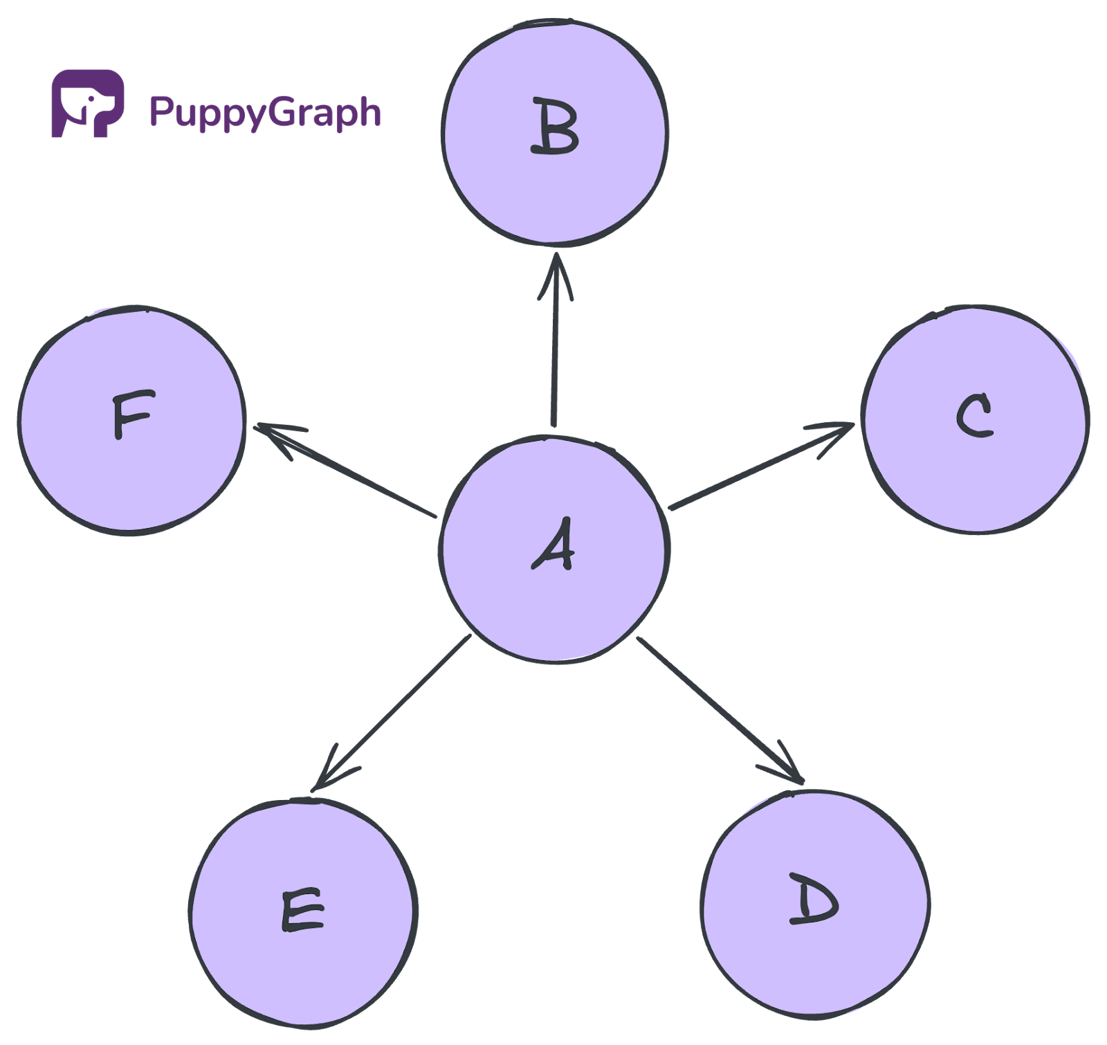
Imagine trying to reach someone through mutual friends. Breadth-first search works by checking everyone one connection away first, then everyone two connections away, then three. In graph terms, BFS explores nodes level by level from the starting point. That is why it is often used when you want the shortest path in an unweighted graph or the nearest matching node.

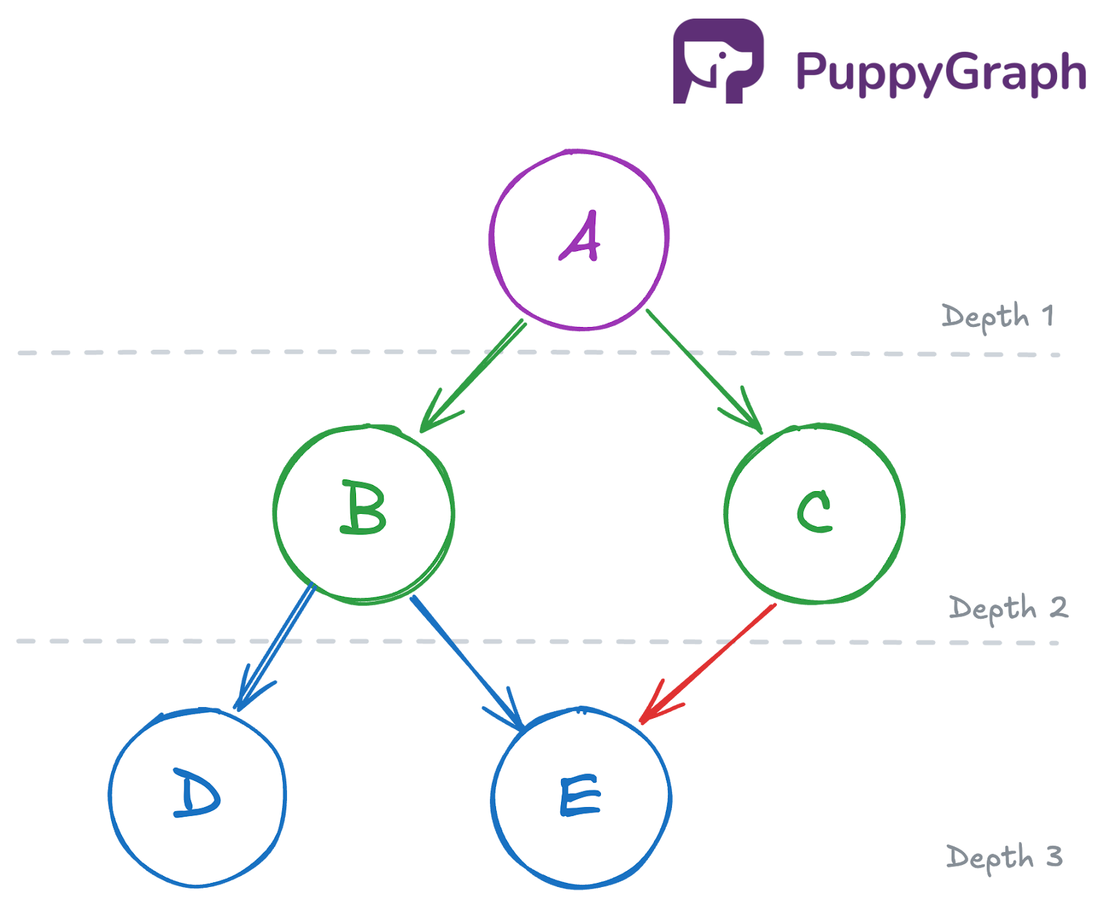
Formally, breadth-first search is a graph traversal algorithm that visits vertices in increasing order of their distance from a source vertex, where distance is measured as the minimum number of edges from the source. In practice, this means BFS processes all nodes at depth 1 before depth 2, then depth 3, and so on. As graphs become more complex, those layers are much harder to see directly, which is exactly where BFS becomes useful.

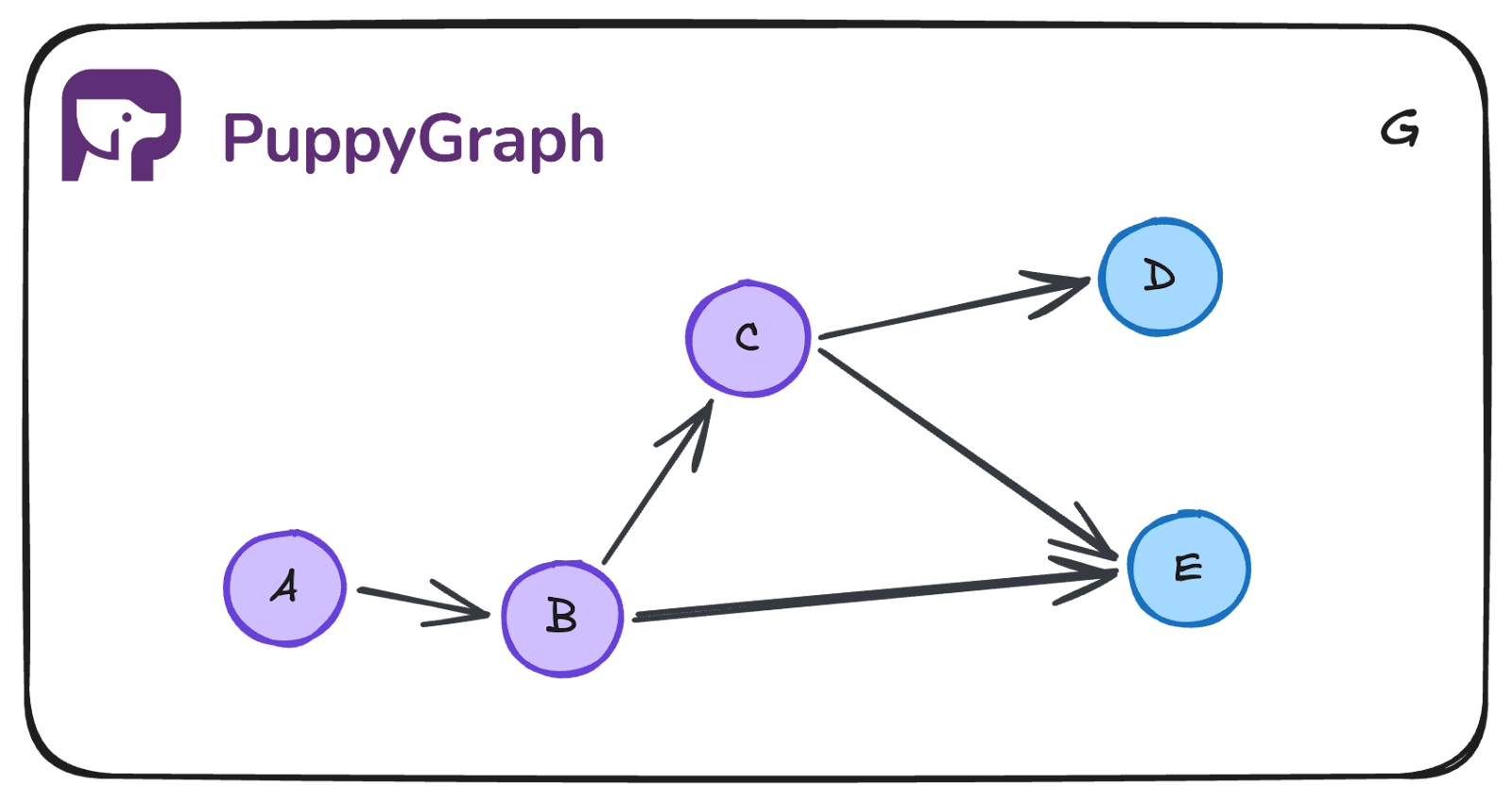
Within each level, the exact visitation order depends on the sequence in which each node’s neighbors are examined. In the simplified example below, B is visited before C simply because B appears first in A’s neighbor list. 

BFS uses a queue to maintain the order. Each newly discovered node is added to the back of the queue, and the next node to visit is taken from the front. This first-in, first-out (FIFO) structure is what gives BFS its characteristic level-by-level behavior.

How Breadth-First Search Works

BFS follows a simple, repeating loop driven by a queue and a visited set. Here’s how it works:

1. Start at the source node. Mark it as visited and add it to the queue.
2. Take the node at the front of the queue and process it.
3. For each neighbor of that node, check whether it has been visited. If it hasn't, mark it as visited and add it to the back of the queue.
4. Repeat steps 2 and 3 until the queue is empty.

Here is a Python example that uses a queue to perform BFS. The focus is on showing the algorithmic structure rather than optimizing performance.

from collections import deque

def bfs(graph, start):
    visited = set([start])
    queue = deque([start])

    while queue:
        node = queue.popleft()  # Dequeue from the front
        print(node)  # Process the node

        for neighbor in graph.get(node, []):
            if neighbor not in visited:
                visited.add(neighbor)
                queue.append(neighbor)  # Enqueue to the back

A node is visited when it is first discovered, marked, and added to the queue. It is processed when it reaches the front of the queue and its neighbors are examined. In other words, a node is always visited before it is processed.

When the queue becomes empty, every node reachable from the source has been visited exactly once, in increasing order of distance from the source.

BFS Example (Step-by-Step)

To see BFS in action, let’s trace it step by step on the same graph from the previous section. 

At each step, we dequeue one node, process its neighbors, and show how the queue changes.

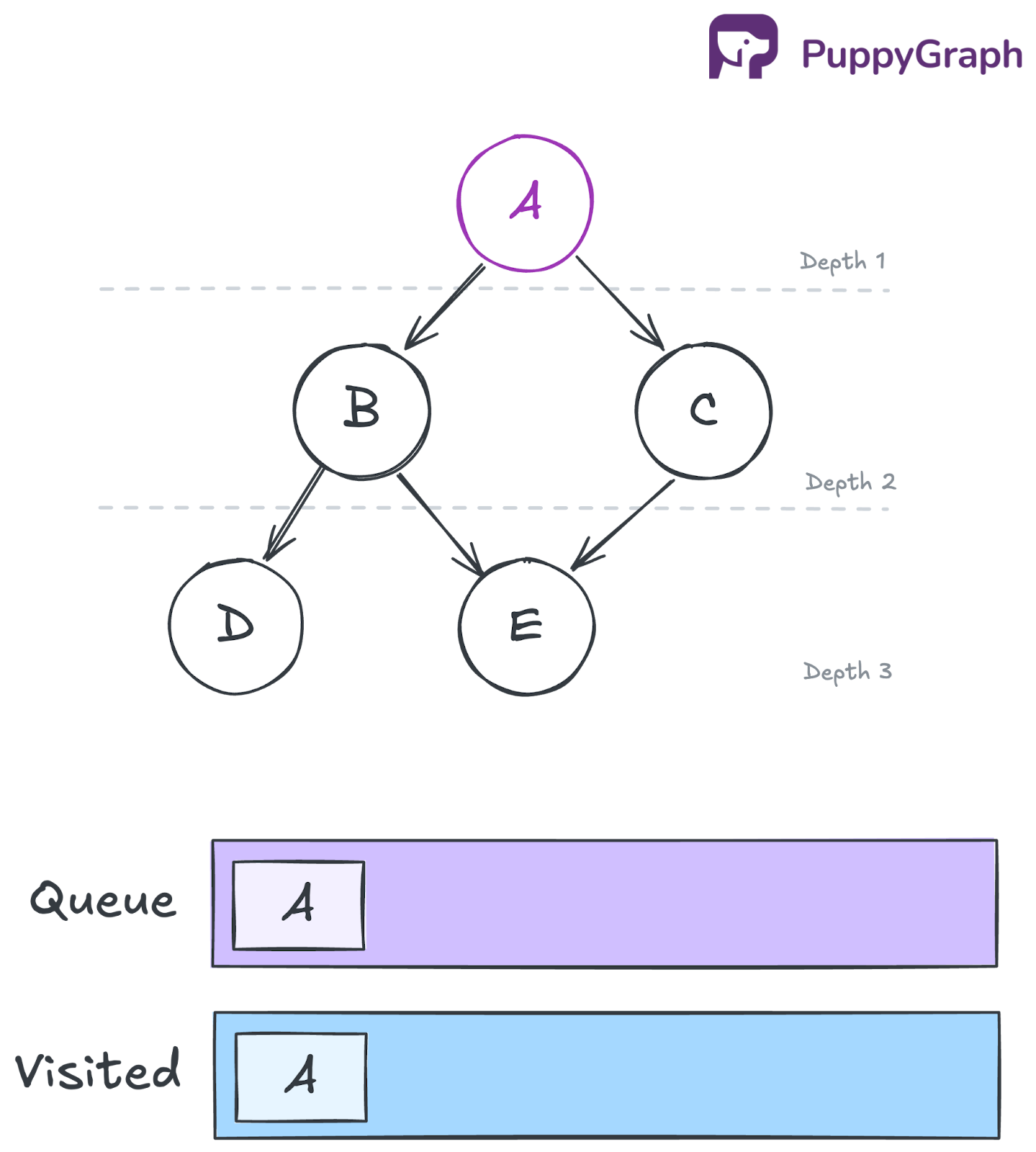
Initialization

Add A to the queue and visited set:

• Queue: [A]
• Visited: {A}
• Traversal so far: []

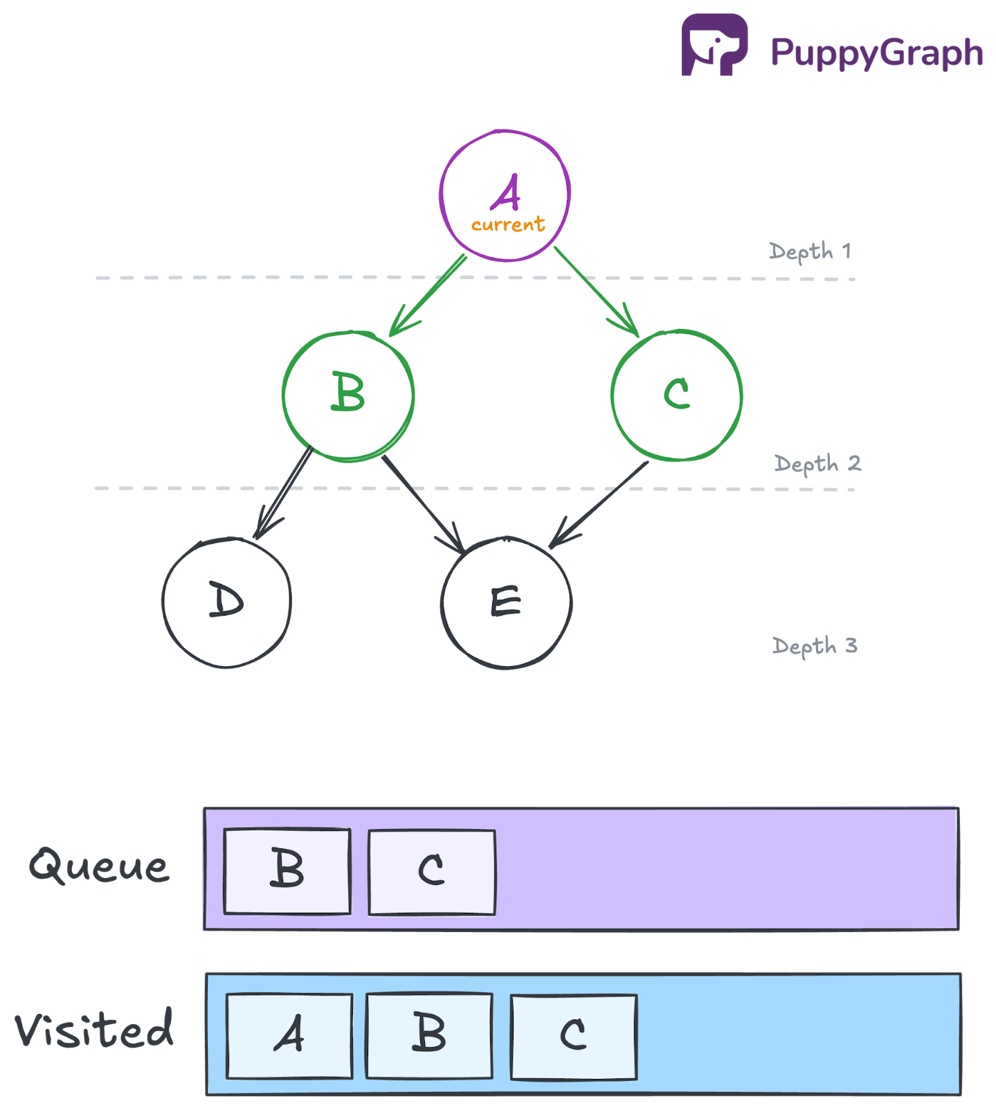
Iteration 1: Dequeue A and process its neighbors

Remove A from the front of the queue and add it to the traversal order. Then inspect A’s neighbors, B and C. Since both are unvisited, mark them as visited and enqueue them.

• Queue: [B, C]
• Visited: {A, B, C}
• Traversal so far: [A]

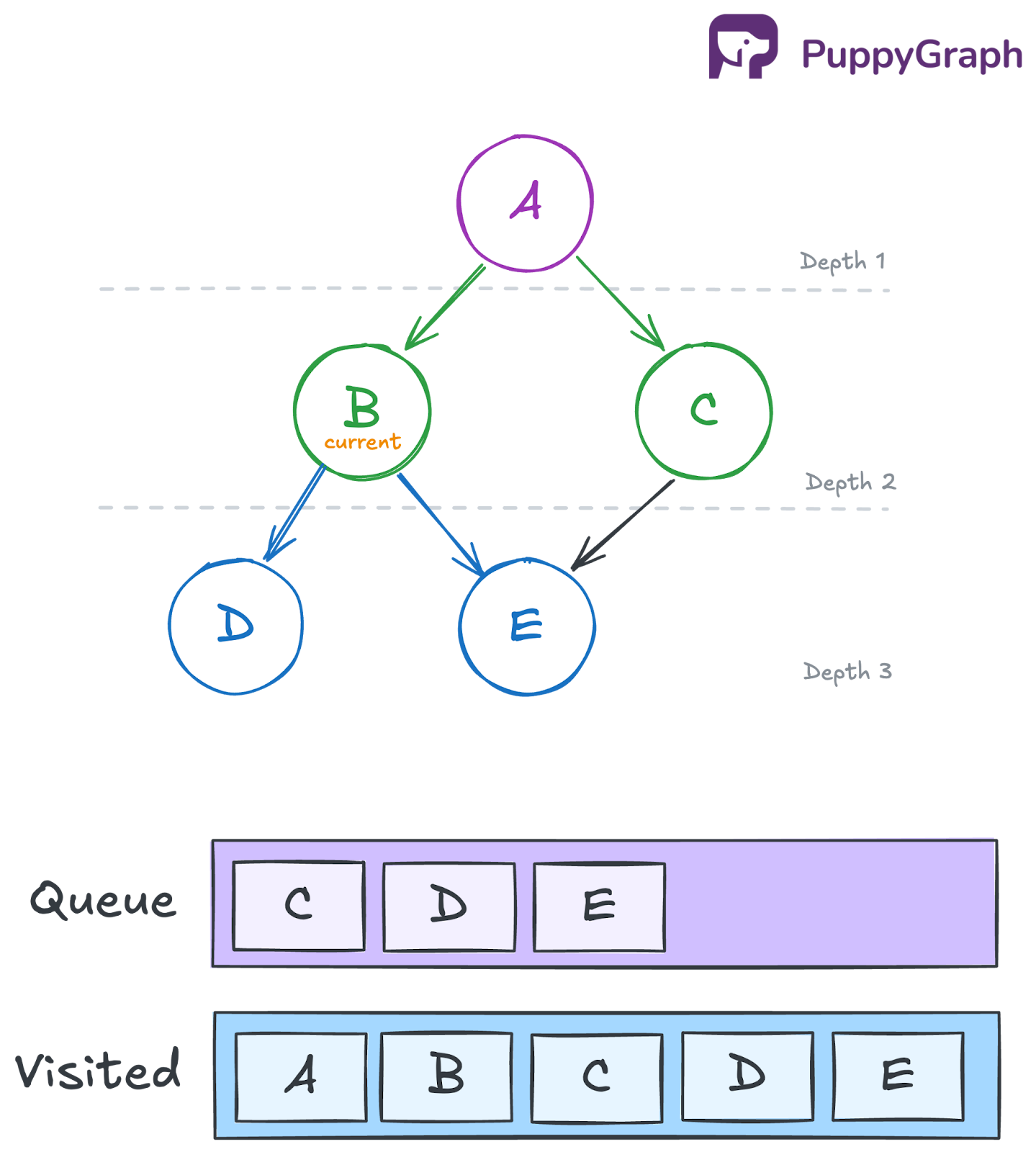
Iteration 2: Dequeue B and process its neighbors

Remove B from the front of the queue and add it to the traversal order. Then inspect B’s neighbors, D and E. Since both are unvisited, mark them as visited and enqueue them.

• Queue: [C, D, E]
• Visited: {A, B, C, D, E}
• Traversal so far: [A, B]

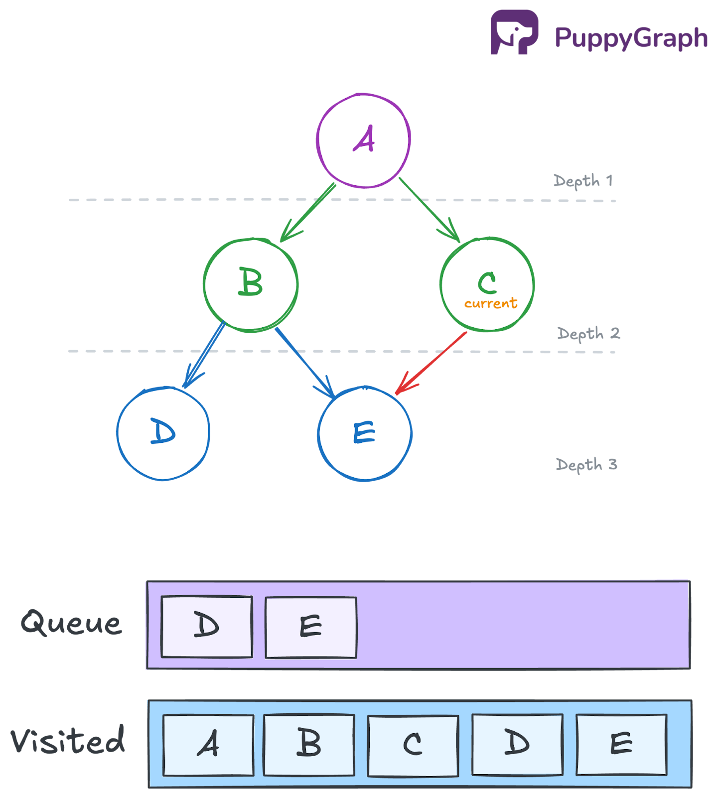
Iteration 3: Dequeue C and process its neighbors

Remove C from the front of the queue and add it to the traversal order. Then inspect C’s neighbors, E. Since E is in the visited set, do not add to the queue.

• Queue: [D, E]
• Visited: {A, B, C, D, E}
• Traversal so far: [A, B, C]

Iteration 4: Dequeue D and process its neighbors

Remove D from the front of the queue and add it to the traversal order. Then inspect D’s neighbors. Since D has no neighbors, no new nodes are added to the queue.

• Queue: [E]
• Visited: {A, B, C, D, E}
• Traversal so far: [A, B, C, D]

Iteration 5: Dequeue E and process its neighbors

Remove E from the front of the queue and add it to the traversal order. Then inspect E’s neighbors. Since E has no neighbors, no new nodes are added to the queue.

• Queue: []
• Visited: {A, B, C, D, E}
• Traversal so far: [A, B, C, D, E]

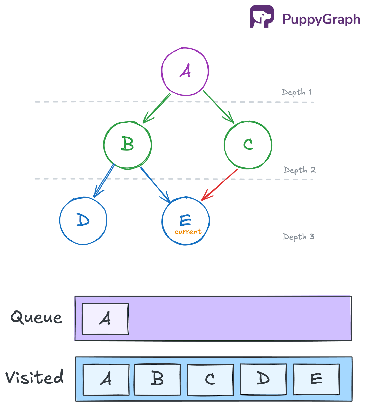
The queue is now empty, so the traversal is complete. The nodes were visited in the order A → B → C → D → E.

Data Structures Used in BFS

BFS relies on two core data structures: a queue to control traversal order and a visited set to avoid revisiting nodes.

The representation of the input graph does not change the algorithm itself, but it does affect the overall time and space complexity.

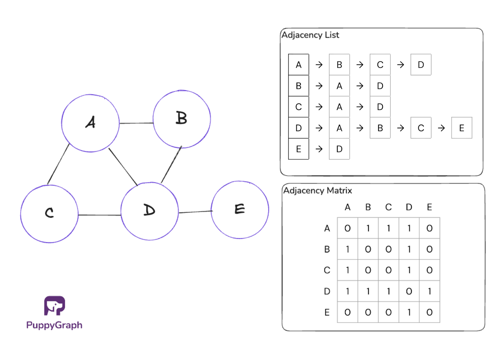
For BFS, adjacency lists are usually preferred because the algorithm spends most of its time iterating through neighbors.

Applications of Breadth-First Search

We leverage BFS when we need to explore a graph outward from a starting point in layers, prioritizing the closest reachable nodes before moving farther away. That makes it a natural fit for the following applications.

Shortest Path in Unweighted Graph

BFS is a standard choice for finding the shortest path in an unweighted graph. Because it explores vertices in increasing order of distance from the source, it finds the fewest-edge path before moving on to longer ones. This makes it useful for problems like maze solving, minimum-move puzzles, and route finding when every step has the same cost.

K-Hop Reachability

Another common use of BFS is k-hop reachability, where the goal is to find all nodes within a fixed number of hops from a source. Because BFS explores the graph layer by layer, it can identify all nodes up to depth \(k\) and stop once that boundary is reached. This makes it useful for neighborhood search, proximity analysis, and bounded exploration in large graphs.

Connected Components

BFS is also commonly used to find connected components in an undirected graph, though DFS works just as well since the goal is simply to traverse every vertex reachable from a starting point. Starting from one unvisited vertex, BFS visits every vertex in that connected region, which forms one complete component. Repeating the process from the next unvisited vertex reveals the next component, and so on. This is useful for identifying isolated clusters, disconnected subnetworks, or separate communities within a larger graph.

Bipartite Graph Checking

A graph is bipartite if its vertices can be divided into two groups such that no edge connects two vertices in the same group. Both BFS and DFS can be used to check this. With BFS, you start from any vertex, assign it to one group, and assign each of its neighbors to the other. As the traversal continues, each newly discovered vertex is placed in the opposite group from the vertex that led to it. If the algorithm ever finds an edge between two vertices in the same group, the graph is not bipartite. If no such conflict appears, the graph can be cleanly divided into two sets.

Advantages of Breadth-First Search

BFS has a few key strengths that make it especially useful in practice. The points below highlight where its traversal order gives it an edge.

• Shortest paths in unweighted graphs: BFS finds minimum-hop paths from a source node. A single run also builds a shortest-path tree to all reachable vertices.

• Reachability and layer discovery: BFS reveals all nodes one hop away, then two hops away, then three, and so on. This makes it useful for k-hop search, connected components, and impact analysis.

• Parallel-friendly traversal: Because BFS explores one layer at a time, many nodes at the same depth can often be expanded simultaneously. That makes BFS practical for large-scale and distributed graph systems.

Disadvantages of Breadth-First Search

BFS also has a few limitations that become important as graphs grow larger or the problem becomes more complex.

• Higher memory usage in practice: While both BFS and DFS have worst-case space complexity of \(O(V)\), BFS often uses more memory because it stores the current frontier, which can grow large in wide graphs. DFS is often lighter in practice because its stack is proportional to the depth of the current path.
  
  
• Not suitable for weighted graphs: BFS only guarantees shortest paths when all edges have equal weight. Once edge weights differ, the path with the fewest edges is not always the path with the lowest total cost, so BFS can no longer be trusted to return the true shortest path.
  
  
• Less efficient when the target is deep: Because BFS visits every node at the current depth before moving deeper, it may spend significant time exploring many nearby nodes even when the target lies far along a single path. In those cases, BFS can become slow and memory-intensive.

Variants of Breadth-First Search

Breadth-First Search also has several useful variants that adapt the same level-by-level traversal idea to different performance needs and search settings.

Parallel BFS

Parallel BFS preserves the same level-by-level logic as standard BFS, but expands many nodes in the same frontier simultaneously. It works especially well when frontiers grow large, which often happens in dense or low-diameter graphs. A low-diameter graph is one where even the most distant pair of nodes is only a few hops apart.

Still, low diameter does not always translate into balanced parallel work. In sparse graphs, or in graphs with highly uneven degree distribution, work can become unevenly distributed across processors.

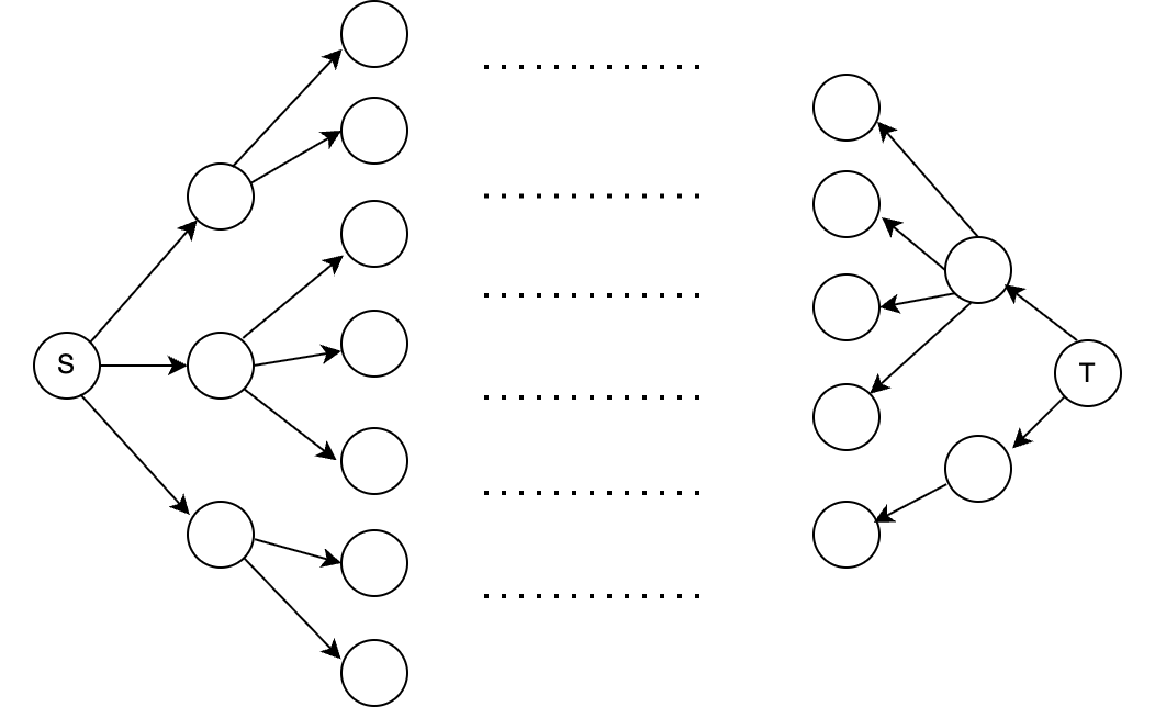
Bidirectional BFS

Bidirectional BFS runs two breadth-first searches at the same time, one from the source and one from the target. Instead of exploring the entire graph outward from one side, the two searches move toward each other. Once a node is found in both visited sets, both sides finish expanding their current level before terminating. This can reduce the search space significantly when both endpoints are known.

This approach can dramatically reduce the search space. In branching-factor terms, a standard BFS explores roughly \(O(b^d)\) states, where \(b\) is the branching factor and \(d\) is the depth of the solution. Bidirectional BFS instead explores roughly \(O(b^{d/2})\) states from each side, assuming symmetric branching.

The key detail is that bidirectional BFS must still preserve BFS’s level-by-level behavior. A correct implementation does not simply alternate between the two queues one node at a time. Instead, it fully expands one current frontier before moving on, often choosing the smaller frontier first to reduce work. This keeps both searches aligned with BFS depth, which is what preserves the shortest-path guarantee in an unweighted graph.

Multi-Source BFS

Multi-source BFS starts from several nodes at once instead of just one. Like standard BFS, each source starts at distance 0, but here all of them are placed into the queue at the beginning so the search expands outward from all sources at the same time. If a node is equally close to multiple sources, the shortest distance is still correct, though which source reaches it first can depend on queue and neighbor ordering.

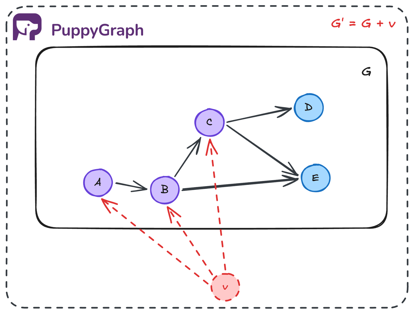
Since multi-source BFS expands from several starting points at once, it is worth asking whether the usual BFS shortest-distance guarantee still holds. A simple way to see that it does is to reduce the problem to ordinary single-source BFS. A useful way to understand this is to imagine adding a virtual super-source \(v\) connected to every source node, creating a new graph \(G’ = G + v\). Standard BFS from \(v\) then behaves the same way as multi-source BFS on \(G\), aside from a one-level offset in distance. This is why the usual shortest-distance guarantee still holds.

Multi-source BFS is useful when you want the shortest distance to the nearest source rather than to one fixed node. Common examples include finding the nearest hospital, server, charging station, or other resource in a graph.

Bonus: Dijkstra’s Algorithm

When it comes to pathfinding, Dijkstra’s algorithm is often described as the weighted extension of BFS rather than a true variant, since it generalizes shortest-path search to graphs with non-negative edge weights. BFS expands nodes in order of increasing hop distance from the source, while Dijkstra’s expands nodes in order of increasing total path cost. When all edges have the same weight, the two produce the same shortest-path results.

Dijkstra’s makes this possible by using a priority queue instead of a FIFO queue. The algorithm is as follows:

1. Assign a tentative distance of 0 to the source node and infinity to all other nodes.
2. Use a priority queue to keep track of which node has the smallest known distance.
3. Repeatedly extract the node with the smallest tentative distance.
4. For each neighbor v of the current node u, compute the cost of reaching v through u. If that cost is smaller than v’s current recorded distance, update v’s distance and insert it into the priority queue, or update its priority if it is already there.

Real-World Use Cases of BFS

In practice, BFS is often used to answer questions about reachability, distance, and nearby relationships in connected data.

Dependency Blast Radius Analysis

In security graphs, BFS is a natural fit for blast radius analysis because it explores outward in order of proximity from a risky starting point. Beginning with a compromised identity, vulnerable asset, or exposed service, BFS identifies the closest connected resources first, then expands to second- and third-hop dependencies. This makes it useful for understanding likely paths of impact and prioritizing the systems that need attention first.

Web Crawlers

In web crawling, BFS provides a useful model for exploring pages in order of proximity from a seed URL. A crawler can begin from one page, visit its outgoing links, then expand to the next layer of pages from there. Real crawlers build on this idea with extra constraints like prioritization, rate limits, and domain-level scheduling, but BFS still captures the core pattern of structured outward exploration.

Recommendation Engines

In graph-based recommendation systems, BFS is often used for candidate generation. Starting from a user, product, or piece of content, it expands outward in order of proximity to surface nearby users, items, or interactions first. This makes it useful for narrowing a large graph down to a relevant local neighborhood before the final recommendation step.

From there, the candidates can be enriched with signals like recency, popularity, similarity, and user preferences, then filtered and re-ranked before they are shown.

Social Network Degrees of Separation

In social networks, BFS is a natural fit for degrees-of-separation analysis because it explores connections in order of proximity from a starting person. Beginning with direct connections, it then expands to friends of friends and the next layers beyond. This makes it useful for measuring social distance, finding connection paths, and identifying who falls within a given social radius.

Conclusion

BFS is simple, but it shows up in more places than it first seems. Once the level-by-level pattern is clear, it becomes easier to see why BFS works for shortest paths in unweighted graphs, why it adapts well to parallel execution, and why bidirectional search can reduce the search space. Most of the variants and use cases in this post follow from that same idea: visit nearby nodes first, then expand outward.

But understanding BFS in the abstract is only part of the story. In practice, the graphs people care about live inside real systems like dependency graphs, user networks, and transaction data, not toy examples. That is where things often get harder. PuppyGraph helps close that gap by letting you run graph queries directly on your existing data sources. With built-in graph traversal algorithms, it lets you run BFS on petabytes of data without moving that data into specialized graph storage.

Want to quickly run BFS on your existing data? Try out PuppyGraph’s forever-free Developer Edition, or book a demo with the team.