Graphs are a natural way to represent relationships, between users, machines, transactions, or any connected entities. A central question in graph analysis is: which parts of the graph are actually connected? In many applications, this isn’t just a structural detail. It determines what’s reachable, what’s isolated, and how information or risk can spread.

The concept of connected components captures this. In an undirected graph, a connected component is a set of nodes where every node is reachable from any other in the same set. Identifying these components is often a first step before deeper analysis like community detection, anomaly tracking, or attack path modeling.

This post explores how connected components are computed. We’ll start with basic graph concepts and walk through the algorithms based on graph traversal and disjoint set union. Finally, we’ll demonstrate how to compute connected components directly on tabular data using PuppyGraph, without data migration or ETL.

Basic Concepts of Connected Components 

Before we can understand what a connected component is, we first have to understand two adjacent concepts: graphs and connectivity.

Graphs

A graph is a set of nodes (also called vertices) connected by edges. It’s a foundational structure for representing relationships—between users, devices, events, or any entities that interact. Following convention, we typically denote the number of nodes by n and the number of edges by m.

Graphs can be undirected, where edges imply mutual relationships (like friendships), or directed, where edges have direction (like who follows whom on a social platform).

In the property graph model, which is widely used in practice, both nodes and edges can carry labels and attributes. For example, a node might represent a user with attributes like name and role, and an edge might represent an access relationship with an associated timestamp. These properties make graphs more expressive and useful in domains like fraud detection, cybersecurity, and infrastructure modeling.

Connectivity

In an undirected graph, connectivity means there is a path between two nodes. If you can get from node A to node B by following a sequence of edges, then A and B are connected.

What are Connected Components?

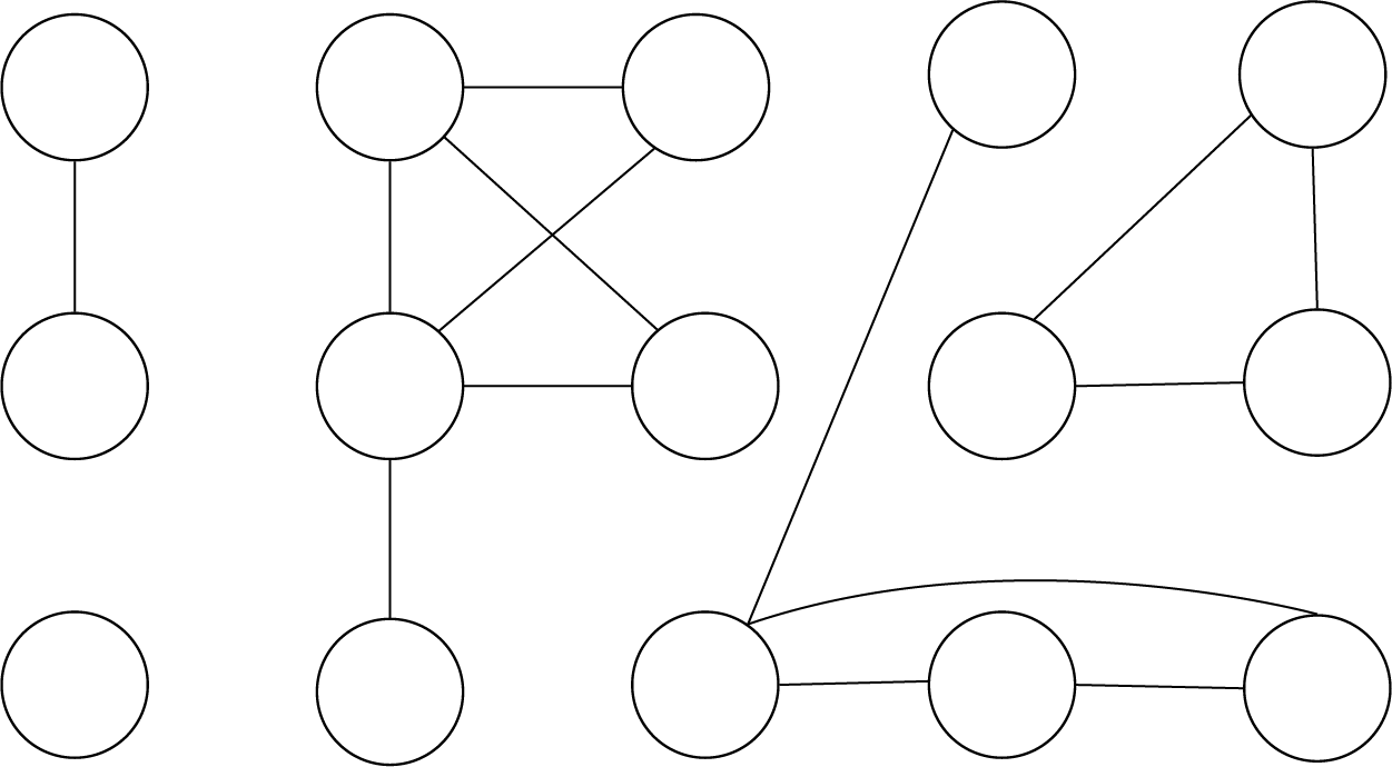
A connected component is a maximal group of nodes where every node is reachable from every other node in the same group. Maximal means that you cannot add any other nodes from the graph and still keep the subgraph connected. Equivalently, there are no edges from the component to nodes outside it. A graph can have one or many connected components.

For a more formal treatment, connectivity can also be defined in terms of vertex cuts. A vertex cut (or separating set) is a set of nodes whose removal increases the number of connected components in the graph. A graph is said to be k-connected if it has more than k vertices and every vertex cut contains at least k nodes. The connectivity of a graph is the largest integer k for which the graph is k-connected.

This formal definition is useful when reasoning about fault tolerance or structural robustness—for example, in network design or critical infrastructure analysis. But in this post, we focus on computing basic connected components: the simpler notion of which nodes are reachable from one another in the graph.

Types of Connected Components

Strongly connected components (SCC)

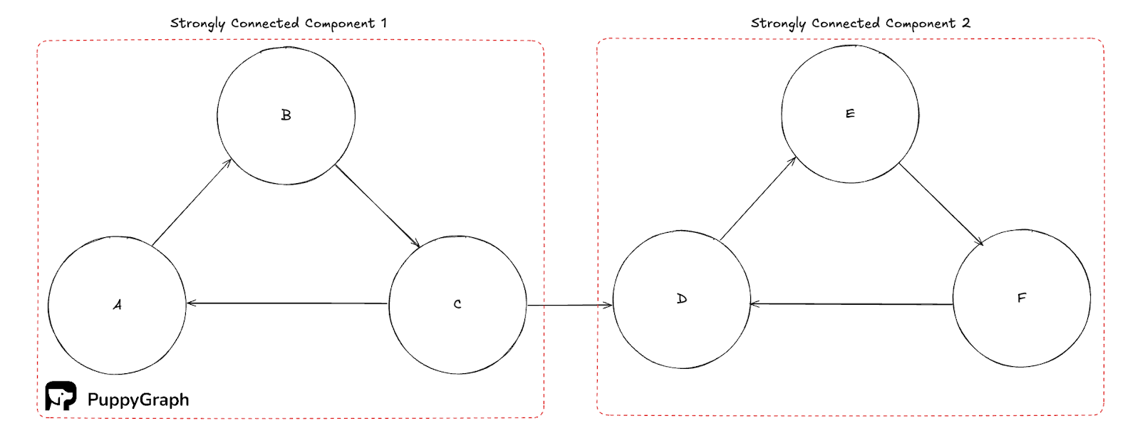
A strongly connected component is a maximal set of vertices in a directed graph where every vertex can reach every other vertex in both directions. While trivial SCCs are just isolated nodes, non-trivial SCCs help to capture tight cyclical structure like feedback loops and mutually dependent services. They partition the graph, and you can find them in linear time with Tarjan’s or Kosaraju’s algorithm, which most libraries expose out of the box.

Weakly connected components (WCC)

A weakly connected component is a maximal set of vertices that is connected if you ignore edge directions. WCCs provide a coarse partition of a directed graph and are often used as a first pass to bound subsequent work. Conceptually, they are the connected components of the graph you get by replacing each directed edge with an undirected one.

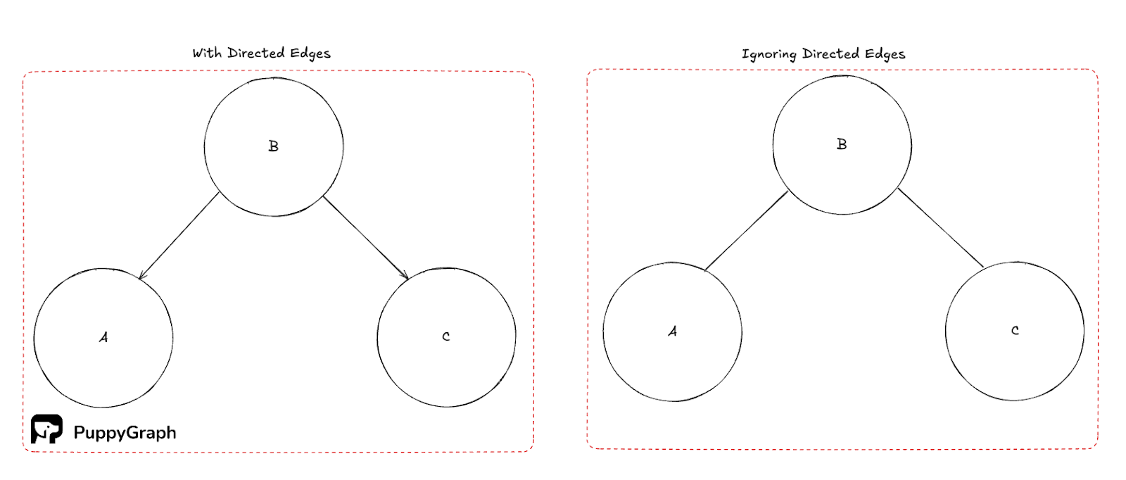
Note that in the figure above, there is no path to Node B unless you ignore the direction of the edges.

Serial Algorithms to Find Connected Components

The simplest way to compute connected components is with a graph traversal. The idea is straightforward: start from a node, explore everything it can reach, and assign all reachable nodes to the same component. Repeat the process for any node that hasn't yet been visited.

DFS and BFS

Both DFS and BFS can be used to explore the graph one component at a time. Here's how it works:

1. Initialize a component ID counter.
2. For each unvisited node:
   
   • Start a DFS or BFS from that node.
   • Mark all visited nodes as belonging to the current component.
   • Increment the component ID.

# Iterative BFS
from collections import deque

def bfs_wcc(graph):
   visited = set()
   components = []

   for start in graph.keys():
       if start in visited:
           continue

       component = set()
       q = deque([start])
       visited.add(start)

       while q:
           u = q.popleft()
           component.add(u)
           for v in graph[u]:
               if v not in visited:
                   visited.add(v)
                   q.append(v)

       components.append(component)

   return components

# Recursive DFS
def dfs_wcc(graph):
   # DFS to get components
   visited = set()
   components = []

   def dfs(u, component):
       visited.add(u)
       component.add(u)
       for v in graph[u]:
           if v not in visited:
               dfs(v, component)

   for u in graph.keys():
       if u not in visited:
           component = set()
           dfs(u, component)
           components.append(component)

   return components

DFS is often used because it's simple to implement recursively, while BFS, though similar in total work, can serve as the basis for parallel algorithms due to its level-based structure. BFS and DFS are useful for finding connected components in undirected graphs, but will not reliably find all SCCs in a directed graph. This is because a single BFS only explores nodes reachable from the starting node, and in a directed graph, reachability is not necessarily symmetric.

Flood Fill Analogy

This process is sometimes compared to flood filling in image processing. Imagine pouring ink on a node: the ink spreads out through all connected nodes, coloring them as part of one component. Then you move to the next unvisited node and repeat. Each flood fill represents one connected component.

Disjoint Set Union (Union-Find)

Another efficient approach is to use the Disjoint Set Union (DSU) data structure, which maintains a partition of nodes into disjoint sets. Initially, each node is its own set. As you process edges, you union the sets of the two endpoints. After all edges are processed, nodes in the same set belong to the same connected component.

The DSU structure supports two operations:

• find(x): returns the representative of the set containing x.
• union(x, y): merges the sets containing x and y.

With path compression and union by rank, both operations run in amortized time O(α(n)), where α is the inverse Ackermann function, a value that grows extremely slowly. In practice, this makes the algorithm effectively constant time for all reasonable input sizes.

‍

With this method, you can process edges in arbitrary order, even when they arrive as a stream. However, similar to DFS and BFS, DSU cannot reliably find all SCCs in a directed graph.

# Disjoint Union-Find (DSU)
from collections import defaultdict

def find(x, parent):
   while parent[x] != x:
       parent[x] = parent[parent[x]]
       x = parent[x]
   return x

def union(a, b, parent, size):
   ra, rb = find(a, parent), find(b, parent)
   if ra == rb:
       return ra
   if size[ra] < size[rb]:
       ra, rb = rb, ra
   parent[rb] = ra
   size[ra] += size[rb]
   return ra

def dsu_wcc(graph):
   # Collect all nodes
   nodes = set(graph.keys())
   for neighbor in graph.values():
       nodes.update(neighbor)

   # DSU tables
   parent = {x: x for x in nodes}
   size = {x: 1 for x in nodes}

   # Union endpoints for each edge (undirected view)
   for u, neighbor in graph.items():
       for v in neighbor:
           union(u, v, parent, size)

   # Gather components by root
   groups = defaultdict(list)
   for u in nodes:
       root = find(u, parent)
       groups[root].append(u)

   return groups.values()

Kosaraju’s Algorithm

Think of Kosaraju as two sweeps over the graph. The first sweep assigns each node a finish time, the second sweep flood-fills on the graph with all edges reversed. Processing nodes in reverse finish order makes each flood fill stay inside one strongly connected component. 

How it works:

1. Run DFS on the original graph. When a node finishes, push it onto a stack or append it to a list.
2. Reverse all edges to build the transpose graph.
3. Initialize a component ID counter.
4. While the stack is not empty, pop a node. If it is unvisited in the reversed graph, start a DFS from it.
5. Mark all nodes reached in this DFS as belonging to the current component ID.
6. Increment the component ID and continue.

# Kosaraju’s Algorithm
def kosaraju_scc(graph):
   # One DFS that can either record finish order or collect a component
   def dfs(u, adjacency, visited, finish=None, comp=None):
       visited.add(u)
       if comp is not None:
           comp.add(u)
       for v in adjacency[u]:
           if v not in visited:
               dfs(v, adjacency, visited, finish, comp)
       if finish is not None:
           finish.append(u)

   # Collect all nodes (keys + neighbors)
   nodes = set(sorted(graph.keys()))
   for neighbors in graph.values():
       nodes.update(neighbors)

   # Build full adjacency for all nodes
   adj = {u: list() for u in nodes}
   for u in nodes:
       adj[u].extend(graph.get(u, list()))

   # Build reversed graph
   reverse_adj = {u: list() for u in nodes}
   for u, neighbors in adj.items():
       for v in neighbors:
           reverse_adj[v].append(u)

   # Pass 1: original graph, record finish order
   visited = set()
   order = list()
   for u in nodes:
       if u not in visited:
           dfs(u, adj, visited, finish=order, comp=None)

   # Pass 2: reversed graph, collect components in reverse finish order
   visited.clear()
   components = list()
   for u in reversed(order):
       if u not in visited:
           comp = set()
           dfs(u, reverse_adj, visited, finish=None, comp=comp)
           components.append(comp)

   return components

Unlike a single DFS or BFS pass, Kosaraju’s two-pass structure means we can reliably find all SCCs since we do not assume that reachability is symmetric.

Tarjan’s Algorithm

The main idea is to run one DFS while tracking two numbers per node:

• index[u]: discovery order of u
  
  
• lowlink[u]: the smallest discovery index reachable from u by zero or more tree edges plus at most one back edge

We maintain a stack of nodes that have been discovered by DFS, but have yet to finish. When lowlink[u] == index[u], u is the root of an SCC, and we’ve identified an SCC. We can then pop the stack up to u, removing all components of this SCC from the stack.

def tarjan_scc(graph):
   discovery = {}       # discovery index per node
   lowlink = {}         # lowlink per node
   stack = []
   on_stack = set()
   components = []

   def strongconnect(u):
       # Use current count of discovered nodes as the next index
       discovery[u] = lowlink[u] = len(discovery)
       stack.append(u)
       on_stack.add(u)

       for v in graph[u]:
           if v not in discovery:         # tree edge
               strongconnect(v)
               lowlink[u] = min(lowlink[u], lowlink[v])
           elif v in on_stack:            # back edge to an open node
               lowlink[u] = min(lowlink[u], discovery[v])

       # Root of an SCC
       if lowlink[u] == discovery[u]:
           component = set()
           while True:
               w = stack.pop()
               on_stack.remove(w)
               component.add(w)
               if w == u:
                   break
           components.append(component)

   # Run DFS from each undiscovered node
   for u in sorted(graph.keys()):       # sorted for deterministic output
       if u not in discovery:
           strongconnect(u)

   return components

Tarjan’s algorithm finds SCCs in a single DFS and can emit components as soon as a root is detected. Compared to Kosaraju’s, this avoids building a transpose graph and keeps memory modest. The tradeoff is that Tarjan is harder to grasp conceptually, since lowlink and the notion of “open” stack nodes are less intuitive than Kosaraju’s two-pass, finish-order approach.

Applications of Connected Components

Entity Resolution and Knowledge Graphs

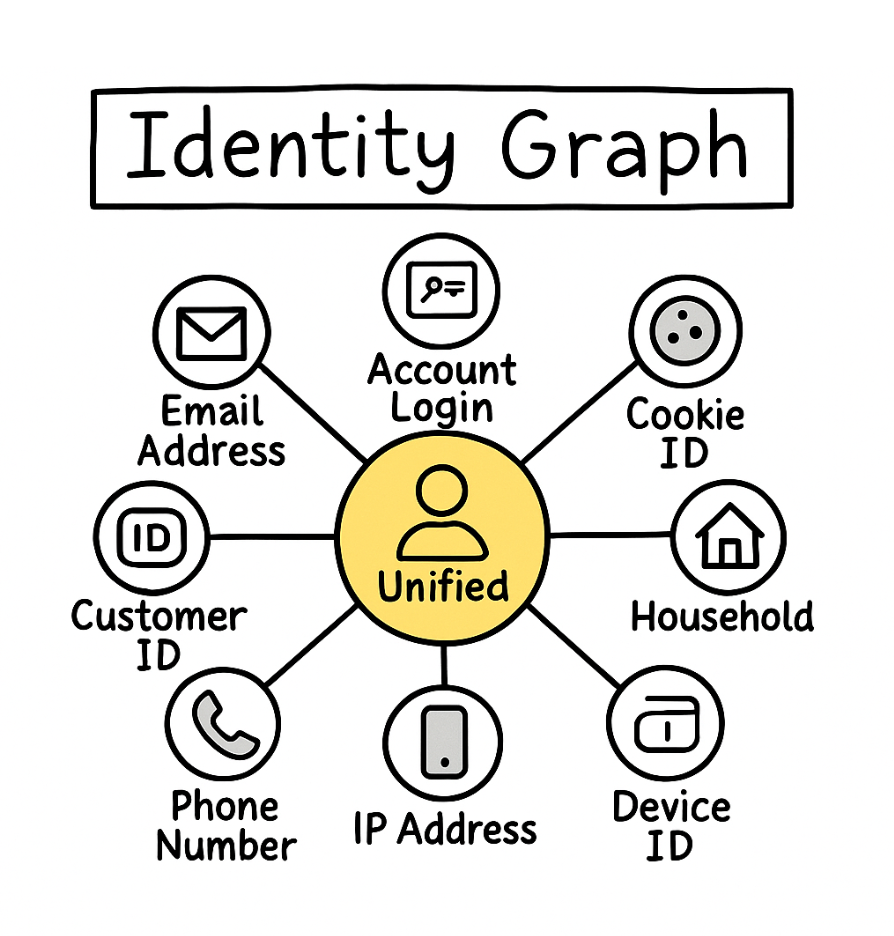
Use weakly connected components to cluster records that refer to the same real-world entity across sources. Build an edge when two records match on evidence such as email, phone, shipping address, or high-confidence fuzzy keys. Each WCC becomes a candidate entity cluster you can score and merge. This approach powers Customer 360, catalog deduplication, identity graphs, and search. It scales well because you can compute WCCs quickly on the undirected view, then apply heavier scoring only inside each cluster.

Fraud Rings

Strongly connected components expose groups where money, credits, or assets can circulate and return to their starting points. Examples include refund triangles, collusive merchants, and account-device meshes that pass value around. SCC size, density, and cycle lengths are useful features for risk models. Once an SCC is flagged, investigators can freeze or step-up verification for the component rather than chasing single nodes. 

Cybersecurity Investigation Scoping

When an alert fires, build a graph of users, hosts, processes, IPs, and events. First compute weakly connected components to bound the blast radius around the indicator, so queries and triage stay inside the relevant subgraph. Inside that region, look for SCCs that suggest command meshes, persistence loops, or automated lateral movement. This WCC-then-SCC pass helps contain query cost, speeds pivots, and highlights feedback structures worth breaking.

Network Reliability and Outage Triage

Treat routers, services, or regions as nodes and links as edges. A spike in the number of weakly connected components signals partitioning. The largest WCC is your surviving core, while small WCCs are isolated islands that need reconnection. For networks with directional constraints, WCCs tell you about basic reachability, and SCCs show where round trips are still possible. This makes it straightforward to localize faults, prioritize restoration, and verify that redundancy plans are working.

Complexity and Performance Analysis

Connected Components In PuppyGraph

Getting started on connected components can feel harder than it should. Real data lives in relational tables, logs, and data lakes. Traditional workflows ask you to copy that data into a specialized graph store, translate schemas, and keep everything in sync with ETL. That means a second storage layer, backfills, broken pipelines, and stale results when jobs miss. The overhead slows teams down and raises costs.

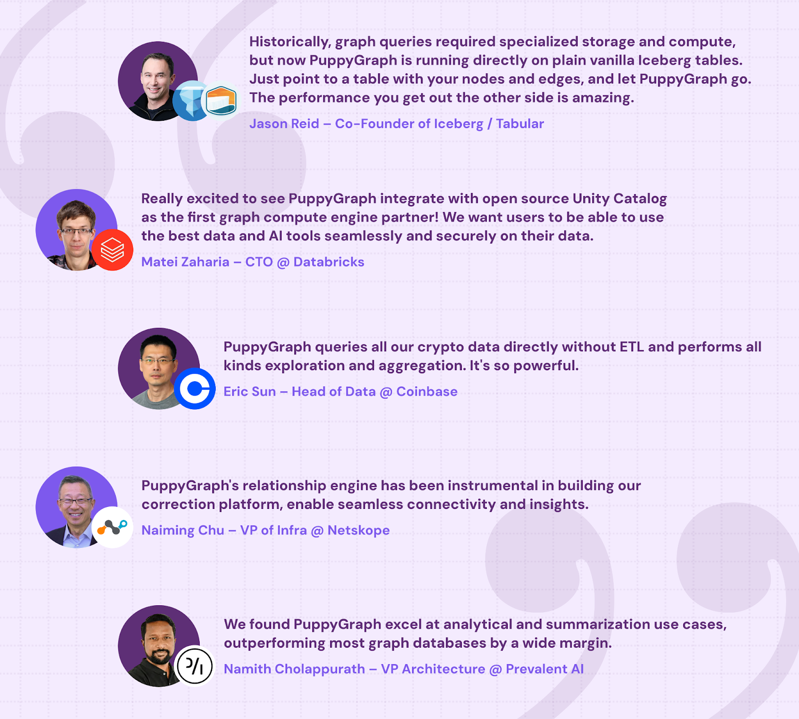
PuppyGraph is the first and only real time, zero-ETL graph query engine in the market, empowering data teams to query existing relational data stores as a unified graph model that deployed in under 10 minutes, bypassing traditional graph databases' cost, latency, and maintenance hurdles. It supports connected component computation directly on top of existing relational data without requiring data movement or ETL. This makes it well suited for production environments where the graph is defined over tables in SQL databases or data lakes, and performance, scale, and ease of use are all important. 

PuppyGraph uses a graph schema to define how tabular data should be interpreted as a graph. The schema specifies which tables represent vertices and edges, how columns map to identifiers and attributes, and how relationships are constructed. After uploading the schema, you can query the graph using openCypher or Gremlin, or invoke built-in algorithms with openCypher or Gremlin syntax.

PuppyGraph provides two built-in algorithms for component analysis and you can see more details in the documentation: Weakly Connected Components (WCC) and Connected Component Finding. These serve different purposes and are suited to different types of graph queries. 

The Weakly Connected Components algorithm identifies all groups of nodes that are connected when edge directions are ignored. This is useful when analyzing directed graphs where directionality may not matter for the purpose of understanding structure—such as identifying isolated user clusters or disconnected subnetworks. The result assigns each node a componentId representing its connected group.

To run WCC, you can use either Gremlin or openCypher syntax. A simple example in Cypher looks like this:

CALL algo.wcc({
  labels: ['User'],
  relationshipTypes: ['LINK']
}) YIELD id, componentId
RETURN id, componentId

For more control, PuppyGraph also supports parameters like maximum iterations, minimum component size, and edge weight filtering.

The Connected Component Finding algorithm, on the other hand, is designed to compute reachability from a given set of start nodes, taking into account edge direction. It returns the set of reachable nodes along with the number of hops from the nearest start node. This is especially useful in exploratory or scenario-based queries, such as “which machines can be reached from a compromised account”.

Here is an example usage in Cypher:

CALL algo.connectedComponentFinding({
  relationshipTypes: ['Knows', 'WorkAt'],
  startIds: ['User[2]'],
  direction: 'BOTH',
  maxIterations: 10
}) YIELD ID, hop
RETURN ID, hop

Both algorithms scale to large datasets and can optionally export results directly to object storage for downstream analysis.

Conclusion

Connected components are a foundational concept in graph analysis. In this post, we walked through several approaches for identifying both weakly and strongly connected components.

PuppyGraph makes it easy to run connected component analysis directly on your relational data, no ETL, no data duplication. Whether you’re working with directed or undirected graphs, you can use high-level queries or built-in algorithms to uncover structure at scale.

Give the PuppyGraph Developer Edition or book a demo to see how it works in action.