What Is GraphX? How Does It Work?

Apache Spark’s GraphX is the graph-computation library built into Spark itself, designed to bring graph algorithms into the same distributed runtime that already handles the rest of an analytics pipeline. Instead of shipping data out to a separate graph system and back, a GraphX job constructs a graph from RDDs, runs operators or message-passing algorithms over it, and joins the results back into whatever DataFrames or downstream stages the application uses. The interesting framing is that GraphX sits at the intersection of two traditions, dataflow systems and graph-parallel computation, and most of its design choices follow from refusing to fully belong to either one.

This post covers what GraphX is and where it currently stands in 2026, the data model and execution style that distinguish it from non-graph Spark code, how its internals partition and route a graph across a cluster, the API surface for constructing a graph, a worked PageRank example, and where it fits relative to other distributed graph options including GraphFrames and engines that query graph-shaped data directly out of existing tables.

What is GraphX?

GraphX is the graph-processing component of Apache Spark. It exposes a property-graph data model, where vertices and edges each carry typed attributes, and provides three things on top of that model: a set of graph-shaped operators (subgraph, mapVertices, aggregateMessages, joinVertices, and so on), implementations of standard algorithms (PageRank, connected components, triangle counting, strongly connected components, shortest paths), and a general-purpose Pregel-style API for defining new iterative algorithms as vertex programs.

GraphX has been part of Spark since the 1.0 release in 2014 and ships with every Spark version, including the 4.2.0 preview released in May 2026. The official Spark documentation still labels GraphX as alpha, which is unusual for a component that has been used in production for more than a decade. In practice the API surface has been stable enough that existing GraphX code keeps working from one Spark release to the next, and the component continues to be built, tested, and shipped alongside the rest of Spark. The longer story behind the alpha label is a question of ecosystem positioning rather than code quality; we come back to it later in the post, after the GraphFrames comparison gives it useful context.

The component is implemented in Scala and exposes its API only to Scala (and, with some friction, Java). There is no first-class Python binding for GraphX, which is the single largest reason teams working primarily in PySpark reach for GraphFrames instead. GraphX is also distinct from a graph database: there is no persistent graph store, no transactional model, no Cypher endpoint. The graph lives only for the lifetime of the Spark job that constructs it. GraphX’s role is graph computation inside a Spark application, not graph storage. The data model is a property graph rather than a labeled property graph: Gaph[VD, ED] applies a single vertex type and a single edge type across the graph, so multi-typed graphs are encoded by making VD a sum type and discriminating at query time, without the first-class labels and relationship types that openCypher and GQL build on.

In practical terms, GraphX is the option to reach for when graph computation needs to run inside an existing Spark pipeline without standing up a separate graph system. The graph is represented as specialized RDDs, and the operators on top of it compose with the ordinary Spark API, so a graph stage can sit between two non-graph stages of the same job without an impedance mismatch at the boundary.

Why graph processing matters

A lot of analytical questions are naturally graph-shaped, and the value of a dedicated graph runtime grows with both the size of the graph and the number of passes an algorithm makes over it. Ranking entities by influence with PageRank on a citation or web graph, finding connected components in a transaction network to surface suspicious clusters, propagating labels across a partially-annotated knowledge graph, counting triangles to estimate clustering coefficients in a social network, computing single-source shortest paths on an infrastructure topology: each of these is an iterative computation that touches every vertex (or every edge) once per pass and converges over many passes. Expressing the same computation in pure SQL forces every iteration to become another self-join over the edge table, and join planners are generally not optimized for long chains of self-joins on a single relation.

Specialized graph systems exist precisely to handle that shape. They store the graph in a form that makes per-iteration access cheap (adjacency lists, columnar edge partitions with per-vertex indexes, compact in-memory layouts), and they expose a computational model where “for every vertex, propagate something to its neighbors, repeat until converged” is first-class rather than emulated on top of a relational engine. The payoff scales with iteration count: a 30-superstep PageRank on a billion-edge graph behaves very differently on a system that keeps the graph resident and indexed across iterations than on one that re-shuffles the edge list each pass.

A useful way to position GraphX inside that space: it is a graph-parallel layer for batch iterative analytics, distinct from a graph database (no persistent store, no transactions) and from low-latency graph query engines (millisecond traversal is not its goal). The next section walks through how it represents a graph and executes those iterations on top of Spark’s RDD machinery.

How GraphX works

GraphX builds three things on top of Spark’s existing RDD machinery: a property-graph data type, a triplet view that joins vertex and edge data on demand, and a Pregel-style message-passing API for iterative algorithms.

Property graph as a distributed data structure.

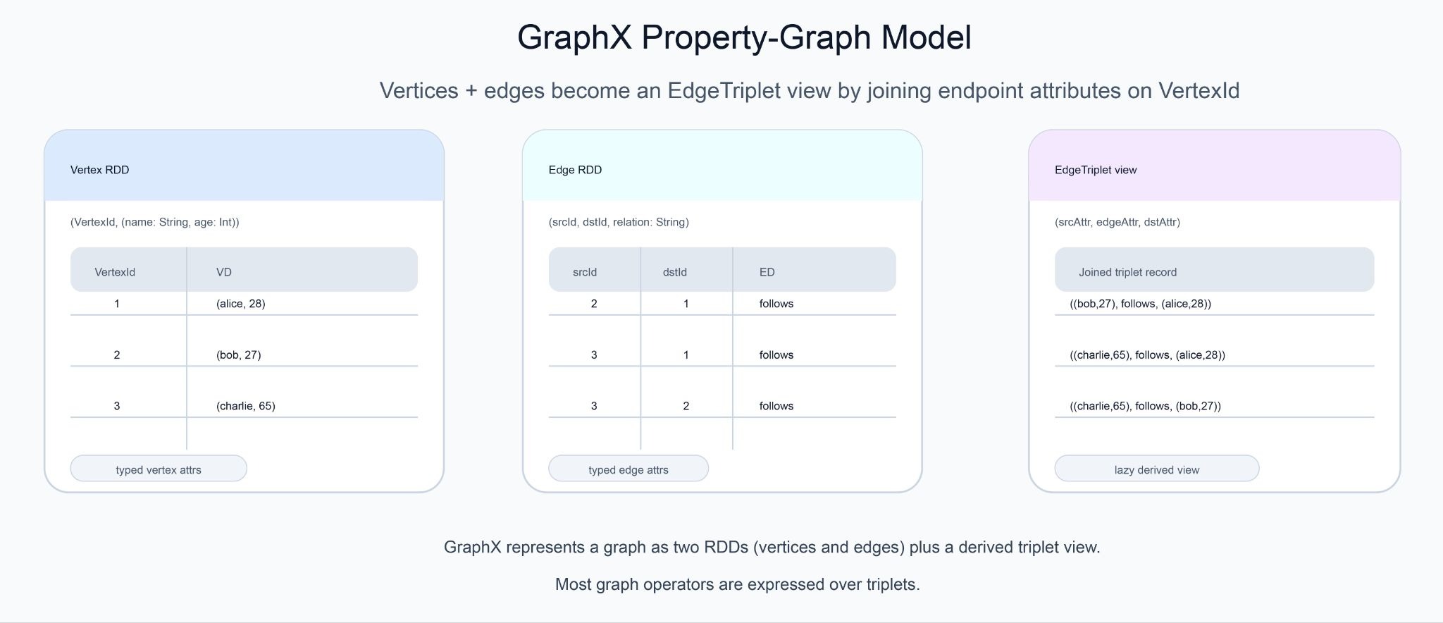
A Graph[VD, ED] in GraphX is a pair of RDDs. The vertex RDD contains (VertexId, VD) pairs, where VertexId is a 64-bit identifier and VD is whatever attribute type the application chooses (a case class, a tuple, a primitive). The edge RDD contains Edge[ED] records, each holding a source id, a destination id, and an ED attribute. Both attribute types are generic, so the same Graph machinery works for a social graph with (name, age) vertices and String edge labels, a financial graph with Account vertices and Transaction edges, or an infrastructure graph with Host vertices and NetworkFlow edges.

The triplet view.

Many graph operations need to look at an edge together with the attributes of both endpoints (the source vertex, the destination vertex, and the edge itself). GraphX expresses this as an EdgeTriplet[VD, ED], conceptually an edge record with the two endpoint vertex attributes joined in. Triplets are materialized lazily and lie at the heart of operators like aggregateMessages, which iterates over triplets and produces a per-vertex aggregate from messages each triplet emits. Most non-trivial GraphX programs are eventually expressible as some shape of triplet aggregation.

Pregel-style message passing. Iterative algorithms like PageRank, single-source shortest paths, and label propagation share a common structure. At each iteration (called a superstep, following the BSP model that underlies Google’s Pregel paper, Pregel: A System for Large-Scale Graph Processing), every active vertex receives the messages sent to it in the previous superstep, updates its own state from those messages, and sends new messages along its outgoing edges. The algorithm terminates when no vertex sends a message or when a maximum iteration count is reached. GraphX exposes this directly through its Pregel API, which takes three user-defined functions: a vertex program, an edge-level message-generation function, and a message-merge function. The built-in implementations of PageRank, SSSP, and connected components are all written against this API and are reasonable reference reading when defining new vertex programs.

The combined effect is that a GraphX program reads like ordinary Spark code with graph-shaped operators layered on top: construct a Graph, transform it with operators, run an algorithm, join the result back to whatever downstream DataFrame or RDD consumes it. Nothing about the surrounding application has to change. The graph-shaped work is just a region of the job.

GraphX architecture explained

The interesting part of GraphX’s implementation is how it makes graph operations efficient on top of an abstraction (RDDs) that was not originally designed with graphs in mind. Three internal mechanisms do most of the work.

VertexRDD and EdgeRDD. Internally, GraphX does not store the graph as two ordinary RDDs. It uses two specialized subtypes, VertexRDD[VD] and EdgeRDD[ED], that maintain extra structure on top of the base RDD: a per-partition index of vertex ids for fast lookup, hash-partitioning of the vertex RDD by id, and a compact in-memory layout for the edge partitions. The result is that operations like joinVertices, which would otherwise require a shuffle, can run partition-local because both sides agree on the partitioning scheme. Reusing the index across stages is one of the main reasons a multi-iteration GraphX algorithm holds up at scale.

Vertex-cut partitioning. A distributed graph can be partitioned in two ways. Edge-cut assigns each vertex to one partition and lets edges cross partition boundaries, which works well for sparse graphs but punishes high-degree vertices. Vertex-cut does the opposite: edges are uniquely assigned to partitions, and vertices are replicated across whichever partitions contain their incident edges. GraphX commits to vertex-cut, on the reasoning (formalized in the GraphX paper, GraphX: Graph Processing in a Distributed Dataflow Framework) that real-world graphs tend to be power-law, with a few high-degree vertices dominating cost. Several partition strategies are available (RandomVertexCut, EdgePartition1D, EdgePartition2D, CanonicalRandomVertexCut), each trading off vertex replication factor against expected communication volume. EdgePartition2D is the default for large graphs because it bounds replication to roughly 2 * sqrt(numPartitions) per vertex.

Routing tables and join optimization. Because vertices are replicated across partitions, GraphX maintains a routing table that records, for each vertex id, which edge partitions hold a replica of it. When an algorithm updates vertex state, the new values can be broadcast only to the partitions that actually need them, instead of shuffling a full copy of the vertex RDD. The routing table is built once when the graph is constructed and reused across stages, which is what makes iterative algorithms like PageRank cheap to run for hundreds of iterations on the same graph.

These three pieces together (specialized RDDs, vertex-cut partitioning, routing tables) are what let GraphX express graph computation as RDD transformations without paying the prohibitive cost of generic distributed joins on every step. The synthesis is worth stating directly: GraphX makes its tightest design commitment by treating Spark’s RDD model as the substrate and absorbing the cost of immutability and lineage, in exchange for fitting naturally into the rest of the Spark ecosystem. Everything that follows in the API, from operator semantics to the Pregel implementation, is a consequence of that decision.

How to create a graph in GraphX

GraphX gives three main ways to construct a Graph, each suited to a different shape of input.

From explicit vertex and edge RDDs. The most flexible constructor takes the two RDDs directly and optionally a default vertex attribute for any vertex referenced by an edge but missing from the vertex RDD.

import org.apache.spark.graphx._
import org.apache.spark.rdd.RDD

val users: RDD[(VertexId, (String, Int))] = sc.parallelize(Seq(
  (1L, ("alice", 28)),
  (2L, ("bob", 27)),
  (3L, ("charlie", 65))
))

val follows: RDD[Edge[String]] = sc.parallelize(Seq(
  Edge(2L, 1L, "follows"),
  Edge(3L, 1L, "follows"),
  Edge(3L, 2L, "follows")
))

val socialGraph: Graph[(String, Int), String] =
  Graph(users, follows, defaultVertexAttr = ("unknown", 0))

From edges alone. When the only meaningful information is the edge structure, Graph.fromEdges and Graph.fromEdgeTuples synthesize the vertex RDD from the unique vertex ids that appear as endpoints, assigning each a constant default attribute. This is the common pattern for unweighted topology analysis like connected components on a raw edge list.

val edges: RDD[Edge[Int]] = sc.parallelize(Seq(
  Edge(1L, 2L, 1), Edge(2L, 3L, 1), Edge(3L, 4L, 1)
))

val topology: Graph[Int, Int] = Graph.fromEdges(edges, defaultValue = 1)

From a text file of edge pairs. The GraphLoader.edgeListFile helper reads a whitespace-separated file of srcId dstId pairs and returns a Graph[Int, Int] with default attributes. This is the path of least resistance for working with the SNAP graph datasets and similar standard benchmark inputs.

val graph: Graph[Int, Int] = GraphLoader.edgeListFile(sc, "data/edges.txt")

Once a graph exists, attributes are reshaped with mapVertices and mapEdges, structural transformations are applied with subgraph, reverse, and mask, and aggregations across edges and their endpoints are expressed with aggregateMessages. The constructors are the entry point. Almost all subsequent work is operator-level.

GraphX example with Apache Spark

A short end-to-end example makes the pieces concrete. The following job builds a small follower graph, runs PageRank to convergence, and joins the resulting ranks back to user names so the output is readable.

import org.apache.spark.graphx._
import org.apache.spark.rdd.RDD
import org.apache.spark.sql.SparkSession

object GraphXPageRank {
  def main(args: Array[String]): Unit = {
    val spark = SparkSession.builder()
      .appName("GraphXPageRank")
      .getOrCreate()
    val sc = spark.sparkContext

    val users: RDD[(VertexId, (String, Int))] = sc.parallelize(Seq(
      (1L, ("alice", 28)),
      (2L, ("bob", 27)),
      (3L, ("charlie", 65)),
      (4L, ("david", 42)),
      (5L, ("ed", 55))
    ))

    val follows: RDD[Edge[String]] = sc.parallelize(Seq(
      Edge(2L, 1L, "follows"),
      Edge(3L, 1L, "follows"),
      Edge(3L, 2L, "follows"),
      Edge(4L, 1L, "follows"),
      Edge(5L, 3L, "follows"),
      Edge(5L, 4L, "follows")
    ))

    val socialGraph: Graph[(String, Int), String] = Graph(users, follows)

    val ranks: VertexRDD[Double] = socialGraph.pageRank(tol = 0.0001).vertices

    val ranksByName = users.join(ranks).map {
      case (id, ((name, _age), rank)) => (name, rank)
    }

    ranksByName.collect()
      .sortBy { case (_, r) => -r }
      .foreach { case (name, r) => println(f"$name%-10s $r%.4f") }

    spark.stop()
  }
}

Running this against a local Spark gives:

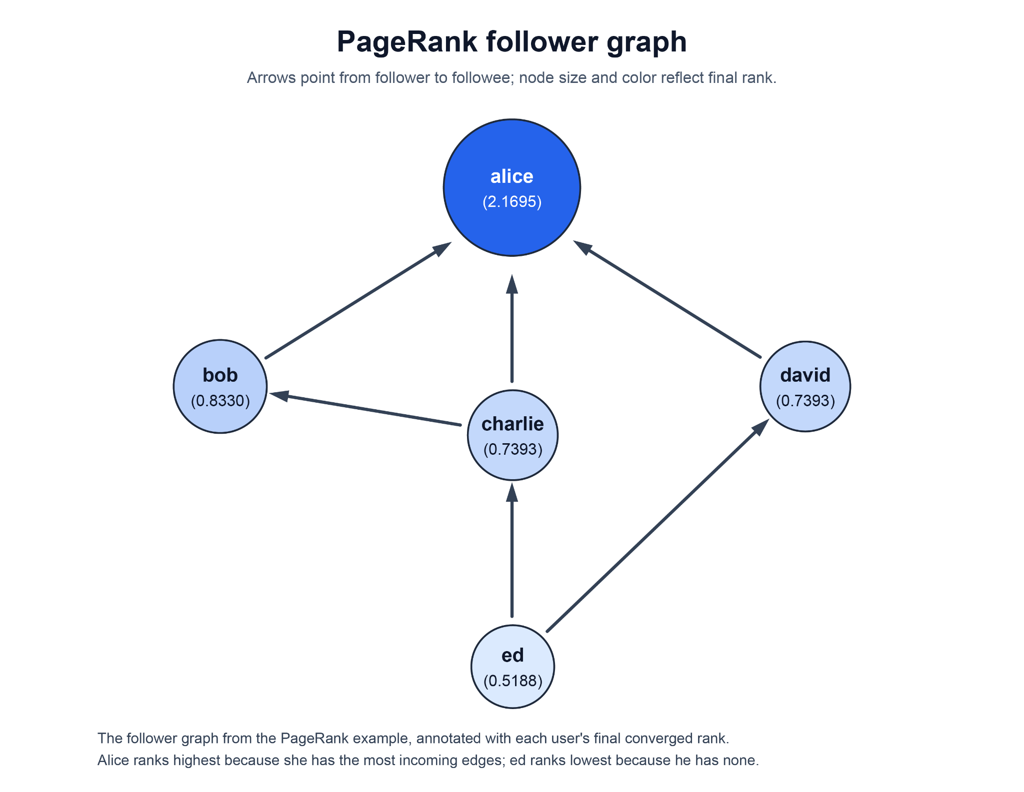
alice      2.1695
bob        0.8330
charlie    0.7393
david      0.7393
ed         0.5188

The ranking lines up with the in-edge structure of the graph. Alice sits at the top because three different users (bob, charlie, and david) follow her, and PageRank concentrates rank wherever incoming edges accumulate. Bob ranks second because he is followed by charlie, who himself carries non-trivial rank from his follower ed. Charlie and david tie exactly because the graph is symmetric around them: each has a single incoming edge from ed and no other in-edges. Ed has no incoming edges at all and so settles at the damping baseline, the lowest stable rank in the network.

A few things in this example are worth reading carefully.

The call socialGraph.pageRank(tol = 0.0001) runs PageRank to a fixed tolerance: the algorithm iterates until no vertex’s rank changes by more than 0.0001 between successive supersteps. The alternative form, staticPageRank(numIter), runs a fixed number of iterations instead, which is preferable when reproducibility across runs matters more than tightness of convergence. The result of either form is itself a graph, with vertex attributes replaced by Double ranks; the example takes the vertices from that result.

The join back to users is doing real work: the rank VertexRDD carries only vertex ids and ranks, not the original (name, age) attributes, so a join is required to make the output human-readable. This pattern (run an algorithm, get a new graph with replaced vertex attributes, join back to original attributes) repeats across almost every GraphX program. It is the analytics equivalent of pivoting back to identifiers after a numerical pass.

Behind the call, PageRank is implemented as a Pregel program. At each superstep, every vertex sends rank / outDegree to each of its outgoing neighbors, sums the incoming messages, and updates its own rank using the standard damping formula 0.15 + 0.85 * sum. On a five-vertex graph the algorithm converges in a handful of iterations; on a billion-edge graph it runs the same code path, with the vertex-cut partitioning and routing tables described earlier doing the work of keeping per-iteration communication bounded.

The shape of this example generalizes. Replace pageRank with connectedComponents, triangleCount, or a custom Pregel program, and the rest of the program stays nearly identical: construct, run, join, surface. Most GraphX code in production is a variation on this pattern, with the construction step usually pulling from much larger inputs than parallelize over a Seq.

GraphX and distributed graph processing

GraphX is one specific point in a wider space of distributed graph systems. Understanding where it sits relative to its neighbors makes the design choices easier to evaluate, and is also the natural place to address the comparison readers reach this post asking about, GraphX vs GraphFrames.

Where GraphX fits among distributed graph engines. When GraphX shipped in 2014, it was one of several Pregel-style systems competing in the open-source distributed graph processing space. Its most-cited peers were Apache Giraph, an open-source port of Google’s Pregel built on Hadoop MapReduce, and Flink Gelly, a graph library that sat on top of Apache Flink’s DataSet API. A decade later that landscape has thinned out considerably. Giraph was retired by the Apache Software Foundation in September 2023 and moved to the Apache Attic in February 2024, where it now sits as a read-only resource. Gelly was tied to Flink’s DataSet API, which was deprecated and then fully removed in the Flink 2.0 release; Gelly itself went with it. GraphX, by contrast, continues to ship with each Spark release because it never had a separate runtime to maintain. Its colocation with the rest of Spark is most of the story: graph computation lives in the same JVM, the same scheduler, and the same RDD lineage as whatever feature engineering or ETL ran before it, so keeping the component building and tested costs the Spark project very little. With the surrounding category of Pregel-style batch graph systems largely absorbed into other paradigms over the same decade, GraphX is best understood as Spark’s RDD-native graph-parallel library rather than a leader in a wider competitive field. How it compares to its DataFrame-based sibling within Spark itself is the question the next subsection takes up.

GraphX vs GraphFrames within the Spark ecosystem. Within Spark itself, the other graph option is GraphFrames, a separately released package maintained primarily by Databricks contributors. The differences are concrete enough to influence project choice.

The persistent alpha label on GraphX is the most-asked-about line in the table, and the comparison is the right place to make sense of it. The label is best read as a stance about the project’s roadmap rather than a comment on quality. GraphX is built entirely on RDDs, and Spark’s main line of development has long since moved to the DataFrame and Dataset APIs and the Catalyst optimizer behind them; with GraphFrames available for DataFrame-shaped graph work, the Spark project has not positioned GraphX as a component to actively expand. The alpha tag tempers the long-term-commitment expectations that would come with promoting it to GA, but it does not amount to a deprecation. GraphX continues to be built, tested, and shipped with every Spark release, and existing code keeps working from one release to the next.

In practical terms the two libraries are not strict replacements. GraphFrames is the natural choice when the broader pipeline is already DataFrame-based and Python is in play, and its motif-finding query language (g.find("(a)-[e]->(b); (b)-[e2]->(c)")) is a meaningful expressivity gain over hand-rolling triplet aggregations in GraphX. GraphX is the natural choice when the algorithm is custom enough to require a Pregel program, when the surrounding code is Scala, or when the constraint that GraphX ships inside Spark itself (no extra dependency, no separate release cadence) matters operationally. For workloads that fall comfortably in the overlap, GraphFrames is usually the lighter starting point and GraphX is the deeper toolkit.

A different architectural path: graph engines that query existing tables. GraphX and GraphFrames both assume the graph step belongs inside a Spark job: read source tables into RDDs or DataFrames at job start, construct the graph in memory, run the algorithm, discard the graph. Every run rebuilds it. A different class of system skips that assembly step and queries graph-shaped data directly out of the warehouse or lakehouse where it already lives. PuppyGraph, used by teams at Palo Alto Networks, Datadog, and Coinbase, is one such engine. It connects to SQL warehouses and lakehouses, maps existing tables to a labeled property graph schema with labels and edge types as first-class concepts rather than the single VD/ED pair GraphX exposes, and serves openCypher and Gremlin queries against the graph. No graph ingestion step, no second copy of the data, no Spark cluster in the path. The underlying tables stay the source of truth and continue serving their other readers in parallel; the graph view is a query-time projection over them rather than a separate dataset. The cut here is workload as much as architecture. The standard graph algorithms (PageRank, connected components, label propagation) are available on both sides; what differs is what each is built around. GraphX is built around batch iterative graph computation, with custom Pregel programs over the full graph as its most distinctive primitive and the algorithm catalog sitting on top of that. PuppyGraph is built around graph querying, with multi-hop traversals and pattern matching in Cypher and Gremlin as its primary surface and the algorithms callable from inside those queries. A custom vertex program that has to sweep a billion-edge graph belongs in GraphX; an entity graph in Iceberg or Snowflake that has to be queried interactively belongs in a query engine over those tables.

Conclusion

GraphX is the part of Spark that takes graph computation seriously enough to design specialized partitioning, indexing, and routing for it, while keeping the result close enough to ordinary RDD code that it composes with the rest of a Spark application. Its data model is a property graph, its execution style centers on the triplet view and the Pregel API, its scaling story rests on vertex-cut partitioning and routing tables, and its API surface is small enough to learn in an afternoon and broad enough to host a wide range of analytical algorithms. In 2026 it remains a current part of Spark, with the alpha label and the absence of Python bindings being the two facts most worth knowing before adopting it.

GraphX is also one option among several. Within Spark, GraphFrames is the natural sibling, DataFrame-based, language-portable, and built around motif finding rather than vertex programs. Beyond Spark, graph query engines that read directly from existing warehouses and lakehouses occupy a different point in the design space, worth evaluating whenever the graph work runs against tables that already live there rather than inside an existing Spark pipeline.

The architectural pattern is easier to evaluate by running it once than by arguing further. Try the forever-free PuppyGraph Developer Edition and book a demo with the team to see how Cypher and Gremlin queries over warehouse and lakehouse tables, with no graph-specific ETL, fit alongside a Spark-based graph step.