Strongly Connected Components : The Ultimate Guide

Graph theory provides a powerful framework for analyzing relationships between objects. Whether modeling social networks, web links, transportation systems, or software dependencies, graphs help reveal how entities interact through connections. Among the many concepts used to analyze directed graphs, strongly connected components (SCCs) play a fundamental role. They help identify clusters of vertices where every vertex can reach every other vertex through directed paths.

Understanding SCCs is particularly useful in large-scale graph analysis, where discovering tightly interconnected structures allows engineers and researchers to simplify complex systems. For example, in program analysis, they expose cycles of mutually dependent functions; and in package management, they uncover circular dependencies that could cause installation issues.

This guide explores strongly connected components from both conceptual and algorithmic perspectives. We will explain what SCCs are, how they appear in directed graphs, and what makes them unique. We will also walk through common algorithms used to compute SCCs, including Kosaraju’s and Tarjan’s algorithms, and discuss how SCCs compare with weakly connected components. By the end of this guide, you will have a solid understanding of SCCs and how they are applied in real-world graph analysis.

What Are Strongly Connected Components?

A strongly connected component is a maximal subset of vertices within a directed graph where every vertex is reachable from every other vertex through directed paths. In other words, if you pick any two vertices within the component, there exists a path from the first vertex to the second and another path from the second vertex back to the first.

This definition highlights the central property of SCCs: mutual reachability. Directed graphs often contain complex pathways where some vertices can reach others but not necessarily return. Strongly connected components isolate the portions of the graph where this bidirectional reachability exists through directed edges.

Strongly connected components essentially divide a directed graph into maximal regions of mutual connectivity. The term “maximal” means that no additional vertices can be included in the component without breaking the reachability property. Each vertex in the graph belongs to exactly one strongly connected component.

SCCs also provide a way to simplify complex graphs. By collapsing each strongly connected component into a single node, we obtain a new graph called the condensation graph, which is always a directed acyclic graph (DAG). This transformation is extremely useful in many algorithms that require acyclic structures. For example, in task scheduling, tasks that depend on each other in a cycle form an SCC, which can be collapsed into a single node. The scheduler can then order these SCCs in the resulting DAG, ensuring all dependencies are respected without getting stuck in cycles.

Strongly Connected Components in Directed Graphs

To understand strongly connected components more formally, we begin with the notion of reachability. In a directed graph, a vertex \(u\) is said to be reachable from a vertex \(v\) if there exists a directed path from \(v\) to \(u\).

Reachability satisfies an important property known as transitivity: if a vertex \(u\) can reach \(v\), and \(v\) can reach \(w\), then \(u\) can also reach \(w\), since the two paths can be concatenated into a single directed path.

Building on this, we define mutual reachability: two vertices \(u\) and \(v\) are mutually reachable if \(u\) can reach \(v\) and \(v\) can reach \(u\). This notion captures bidirectional connectivity in directed graphs.

Mutual reachability satisfies three important properties:

• Reflexivity: every vertex can reach itself,
• Symmetry: if \(u\) and \(v\) are mutually reachable, then \(v\) and \(u\) are also mutually reachable,
• Transitivity: if \(u\) and \(v\) are mutually reachable, and \(v\) and \(w\) are mutually reachable, then \(u\) and \(w\) are also mutually reachable.

Therefore, this relation is an equivalence relation on the set of vertices.

As a consequence, the graph can be partitioned into disjoint equivalence classes under this relation. Each equivalence class forms a maximal set of vertices that are mutually reachable, which is precisely a strongly connected component (SCC). Vertices in different classes are not mutually reachable. 

In addition, if two vertices are mutually reachable, then every vertex on any path between them must also belong to the same SCC. To see this, assume \(x\) and \(y\) are mutually reachable, and there exists a path from \(x\) to \(y\) that passes through a vertex \(z\). Clearly, \(x\) can reach \(z\), and \(z\) can reach \(y\). Since \(y\) can reach \(x\), it follows that \(y\) can reach \(z\) via \(y \to x \to z\). Thus, \(z\) and \(y\) are mutually reachable, and therefore \(z\) belongs to the same SCC as \(x\) and \(y\).

To better understand the algorithms in the subsequent sections, it helps to first look at how directed graphs are explored.

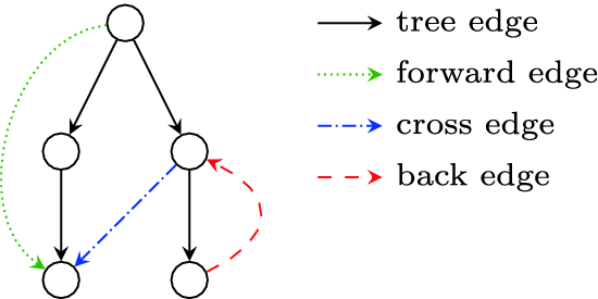
A key tool is depth-first search (DFS). When DFS runs on a graph, it explores as far as possible along each path before backtracking, forming a structure known as a DFS tree. During this process, edges can be classified into four types:

• Tree edges, which are used to first discover new vertices
• Back edges, which point to an ancestor in the DFS tree
• Forward edges, which point to a descendant
• Cross edges, which connect different branches of the traversal

Among these, back edges are especially important, because they indicate the presence of cycles. Since strongly connected components are closely tied to cycles and mutual reachability, this DFS structure provides the foundation for identifying them.

Key Features of Strongly Connected Components

As we discussed in the previous section, strongly connected components form a partition of the graph. If two vertices are both strongly connected to a third vertex, then by transitivity they are also strongly connected to each other, meaning they must belong to the same component. As a result, no vertex can belong to more than one SCC.

Furthermore, each component is maximal with respect to this property. If there were a vertex outside the component that could both reach and be reached from all vertices inside it, transitivity would force it to be included in the same group. Therefore, SCCs capture the largest possible regions of mutual reachability.

Another key implication is that cycles are fully contained within strongly connected components. Any cycle ensures mutual reachability among its vertices, and through transitivity, overlapping cycles merge into a single SCC. In this way, SCCs can be seen as the natural “containers” of cyclic structure in directed graphs.

Finally, when each SCC is collapsed into a single node, the resulting graph contains no cycles. If a cycle existed between components, it would imply mutual reachability across them, contradicting their maximal separation. Therefore, the condensation graph must be a directed acyclic graph (DAG), revealing a higher-level structure where components depend on one another without forming loops.

Example of Strongly Connected Components in a Graph

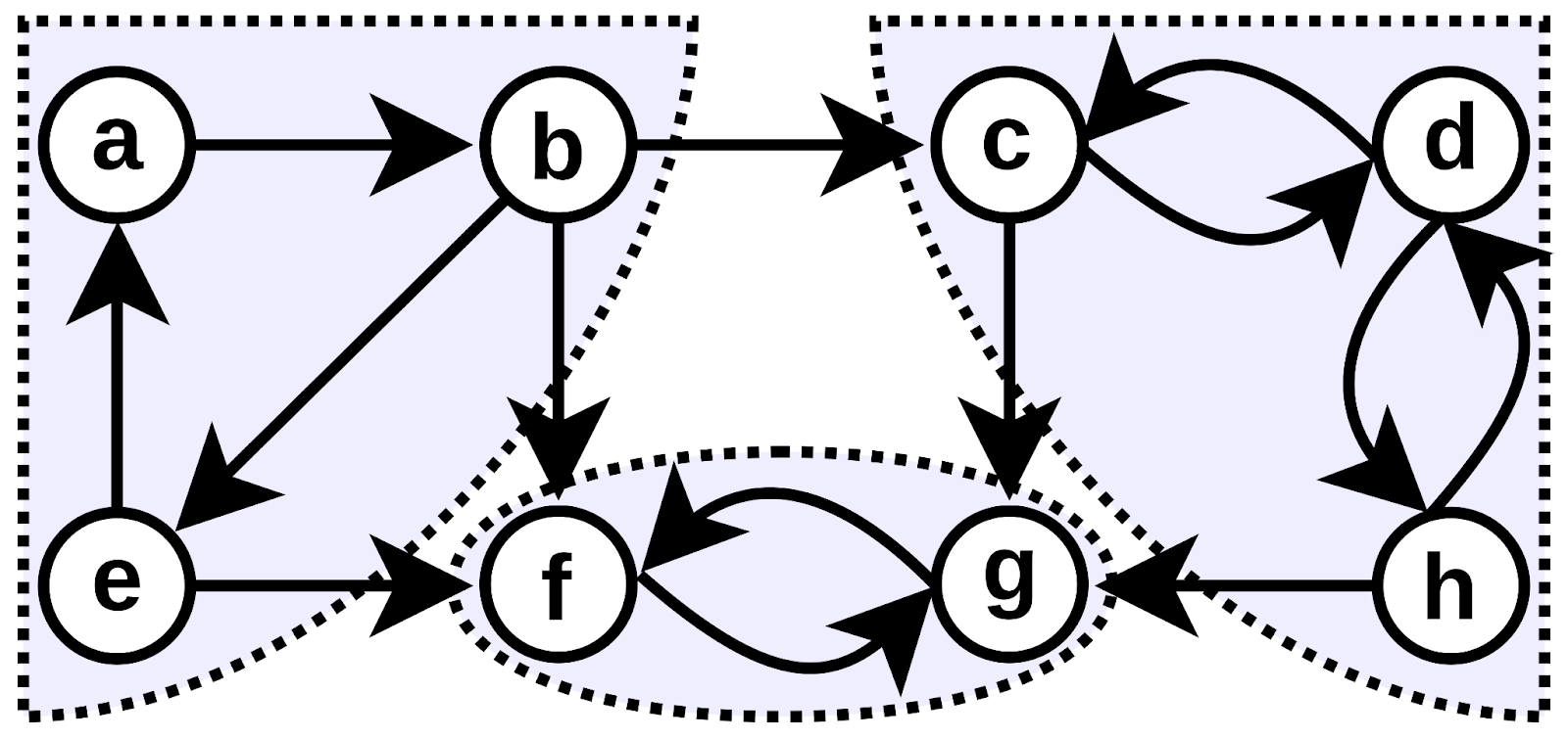
To better understand how strongly connected components arise in more realistic settings, consider the following directed graph:

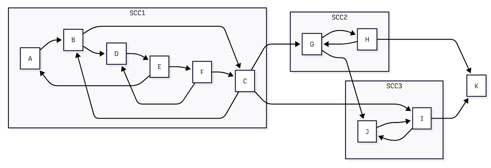
The figure above illustrates a directed graph with multiple strongly connected components (SCCs). Each SCC is a maximal set of vertices in which every vertex can reach every other vertex in the same set.

SCC1 (A, B, C, D, E, F):
This large component contains six vertices. Despite the complex internal structure, every vertex can reach every other vertex via some directed path. For example, you can start at A and eventually reach F, and from F you can return to A following a different path. This mutual reachability binds all six vertices into a single SCC.

SCC2 (G, H):
Vertices G and H form another strongly connected component. Both vertices are mutually reachable, but they are separate from SCC1 because there is no path from SCC2 back to SCC1.

SCC3 (I, J):
Vertices I and J form a third SCC. These two vertices are mutually reachable, but they cannot reach SCC1 or SCC2, so they remain a distinct component.

K:
Vertex K is reachable from SCC2 and SCC3, but since no paths return to either component, K forms a trivial strongly connected component by itself.

Inter-Component Connections:

• SCC1 → SCC2: The path from C to G allows traversal from SCC1 to SCC2, but the lack of a return path ensures that SCC1 and SCC2 remain separate SCCs.
• SCC1 → SCC3: Similarly, C → I connects SCC1 to SCC3 unidirectionally.
• SCC2 → SCC3: G → J connects SCC2 to SCC3, but no reverse path exists.
• SCC2 → K and SCC3 → K: Paths H → K and I → K lead to the trivial SCC formed by vertex K.

These directed connections highlight that while one SCC may reach another, mutual reachability across components does not exist, preserving the distinction between SCCs.

Algorithms Used to Find Strongly Connected Components

Detecting strongly connected components efficiently is an important task in graph theory and computer science. Several algorithms have been developed for this purpose, with most operating in linear time relative to the number of vertices and edges.

Two of the most widely known algorithms are Kosaraju’s algorithm and Tarjan’s algorithm. Both rely on depth-first search (DFS) but approach the problem in different ways.

Kosaraju’s Algorithm

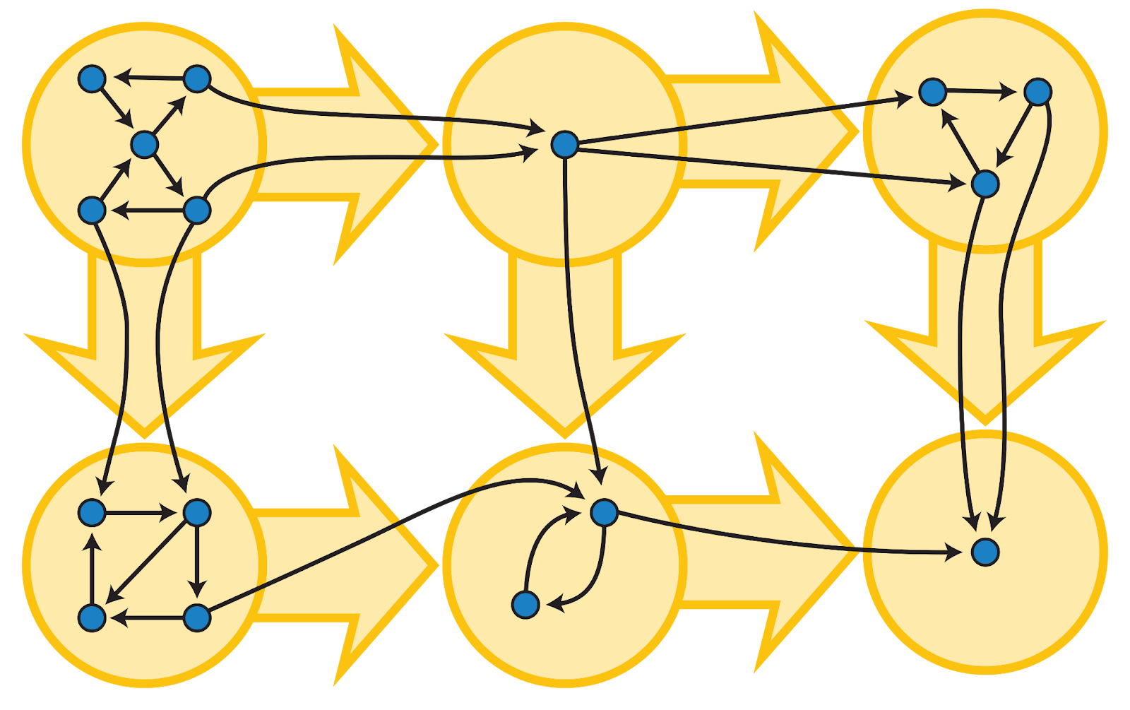
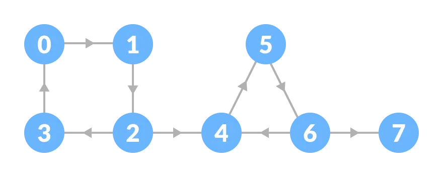
Kosaraju’s algorithm is conceptually simple and works in two passes of depth-first search. In the first pass, DFS explores the graph and records the order in which vertices finish processing, where a vertex’s finishing time is the moment when all vertices reachable from it have been fully explored and the search backtracks. Consequently, vertices deeper in the DFS recursion finish earlier: for example, in the figure below, \(3\) finishes first, followed by \(7\), \(6\), \(5\), \(4\), \(2\), \(1\), and finally \(0\).

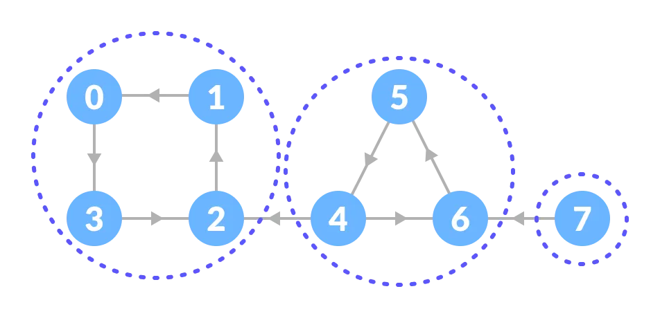
Next, the algorithm constructs the transpose graph, where every edge is reversed. Running DFS again on the transposed graph, but processing vertices in decreasing order of their finishing times. Each DFS traversal in this second phase identifies one strongly connected component. The algorithm continues until all vertices have been visited.

Kosaraju’s algorithm is easy to understand and implement. However, it requires constructing the transposed graph and performing two DFS passes, which can increase memory usage in very large graphs.

Correctness

The correctness of Kosaraju’s algorithm is based on the following facts:

1. If we call the maximum finishing time among all vertices in an SCC its finishing time, then these finishing times determine a topological ordering of the SCCs.
2. After reversing all edges, performing DFS in decreasing order of finishing times ensures that each DFS traversal visits exactly one SCC.

Complexity

Kosaraju’s algorithm performs two DFS passes and constructs the transpose graph, so it runs in linear time relative to the number of vertices and edges, \(O(V + E)\). While simple and intuitive, it may use additional memory for the transposed graph in very large graphs.

Tarjan’s Algorithm

Tarjan’s algorithm finds strongly connected components (SCCs) in a graph using depth-first search (DFS). The algorithm maintains an auxiliary stack \(S\), and each vertex \(v\) is assigned a unique index \(dfn(v)\), numbering the vertices consecutively in the order in which they are discovered. The algorithm also maintains a “lowlink” value \(low(v)\) for each vertex \(v\), which represents the smallest index of any vertex on the stack \(S\) that is reachable from \(v\) through its DFS subtree by one edge, including \(v\) itself.

When a vertex \(v\) is visited, its \(dfn(v)\) is assigned and \(v\) is pushed onto the stack \(S\). After the DFS processing of \(v\) is completed, its lowlink value \(low(v)\) is determined. At this point, if \(dfn(v) = low(v)\), then \(v\) is the root of a strongly connected component. The vertices in this SCC are exactly those on the stack \(S\) from the top down to \(v\). The algorithm then repeatedly pops vertices from the stack until \(v\) is removed.

This approach ensures that vertices belonging to the same SCC are contiguous on the stack, and each SCC is output exactly once.

Correctness

When running Tarjan’s algorithm, suppose we are currently processing a vertex \(x\) and consider the stack \(S\). Vertices in \(S\) can be viewed in two groups.

First, vertices still in the DFS recursion stack (i.e., not yet finished). These are exactly the ancestors of \(x\) in the DFS tree.

Second, vertices whose DFS has finished but are still kept in \(S\). For any such vertex \(y\), we must have \(low(y) < dfn(y)\); otherwise, if \(low(y) = dfn(y)\), \(y\) would have already been popped as the root of an SCC.

Now take any vertex \(z \in S\). There must be a path from \(z\) to some ancestor of \(x\). If \(z\) is an ancestor, this is trivial. Otherwise, since \(low(z) < dfn(z)\), we can follow a chain of vertices with strictly decreasing \(dfn\) values until we reach an ancestor of \(x\).

This implies a key property: if there is an edge \(x \to y\) and \(y \in S\), then \(x\) and \(y\) are in the same SCC.

From here, we can interpret \(low(x)\) as the smallest discovery time reachable from the subtree of \(x\) by one edge within its SCC. In particular:

• \(low(x) < dfn(x)\) means \(x\) can reach an earlier vertex in its SCC
• \(low(x) = dfn(x)\) means \(x\) is the earliest (root) vertex in its SCC

Now suppose we finish exploring the subtree of \(x\) and still have \(low(x) = dfn(x)\). Let \(T\) be the segment of the stack from the top down to \(x\).

Every vertex \(y \in T\) lies in the subtree of \(x\) and remains in the stack, so it can reach back to \(x\), implying \(y\) and \(x\) are in the same SCC.

Conversely, any vertex in the subtree of \(x\) but not in \(S\) must have been popped earlier as part of another SCC, so it cannot belong to \(SCC(x)\).

Therefore, \(T\) is exactly the strongly connected component of \(x\).

Complexity

Because Tarjan’s algorithm processes each edge and vertex only once, it runs in \(O(V + E)\) time complexity, where \(V\) is the number of vertices and \(E\) is the number of edges. Its efficiency and single-pass design make it a popular choice in many graph processing libraries.

Strongly Connected Components vs Weakly Connected Components

In graph theory, the concept of connectivity differs depending on whether the graph is directed or undirected. Strongly connected components represent one form of connectivity in directed graphs, but another concept known as weakly connected components also exists.

A weakly connected component is a set of vertices that become connected when edge directions are ignored. In other words, if we treat every directed edge as an undirected edge, a weakly connected component includes all vertices that can reach one another through some path.

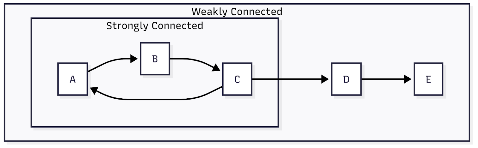
This difference leads to distinct interpretations of graph structure. In strongly connected components, direction matters: vertices must be mutually reachable following the direction of edges. In weakly connected components, direction is irrelevant, and connectivity simply means there is some path between vertices.

In the figure above, vertex C points to D and D points to E, but no edges point back. In this case, all these three vertices belong to the same weakly connected component because ignoring direction reveals a connected structure. However, they cannot form a strongly connected component together, since there are no return paths.

Understanding the difference between these two concepts is important when analyzing real-world networks. Strong connectivity reveals feedback loops and cyclical relationships, while weak connectivity reveals broader structural groupings.

Both types of connectivity provide valuable insights depending on the goals of the analysis.

Conclusion

Strongly connected components provide a fundamental way to understand the structure of directed graphs by identifying maximal groups of vertices with mutual reachability. By partitioning a graph into SCCs and analyzing the resulting condensation graph, complex systems can be simplified into clear, acyclic structures. This perspective not only clarifies how cycles are formed but also reveals higher-level dependencies between different parts of a graph.

In practice, SCCs are essential for analyzing real-world systems such as software dependencies, network structures, and program execution flows. Algorithms like Kosaraju’s and Tarjan’s enable efficient detection of these components in linear time, making them practical even for large graphs. Together, the theory and algorithms of SCCs provide powerful tools for both understanding and solving problems in graph-based applications.

Explore more with the forever-free PuppyGraph Developer Edition, or book a demo to see it in action.