What Is Data Mining? Techniques, Examples & Uses

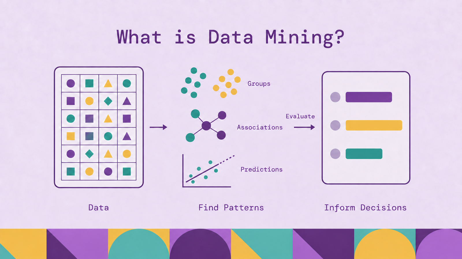
Data mining helps businesses find patterns they can use to make decisions: which customers may leave, which products tend to sell together, or which transactions deserve investigation. Its value depends on whether those patterns hold beyond the records that first revealed them and support a useful action.

This guide explains how data mining works, the steps involved, and the main techniques. It also walks through practical examples, business applications, and the limitations that determine whether a promising result becomes a dependable part of operations.

What is data mining?

Data mining is the analysis of datasets to discover useful patterns, relationships, and predictive signals. It draws on statistics, machine learning, and database methods. The output might be a prediction model, a set of association rules, a grouping of similar records, or a shortlist of unusual events. IBM's overview of data mining distinguishes descriptive methods, which characterize existing data, from predictive methods, which estimate outcomes.

Consider a retailer's transaction history. Reporting can establish how much revenue each store generated. Data mining can examine whether particular purchase combinations recur or whether changes in buying behavior help predict a customer's next purchase. Both activities use the same records, but they ask different questions.

Machine learning supplies many of the algorithms used in data mining. A data mining project also requires deciding which records belong in the analysis, interpreting what the output means, and checking whether the finding matters to the business. Training an algorithm is one part of that work.

The dataset need not be enormous. A smaller collection of well-defined observations may answer a focused question more reliably than a much larger collection with inconsistent identifiers, missing outcomes, or irrelevant attributes.

How does data mining work?

Data mining works by representing observations in a form that an analytical method can compare, then searching for structure according to that method's objective. The representation determines which patterns the method can see.

For a subscription business, one observation might be an account at the start of a month. Its attributes, called features, could include recent usage, subscription tenure, and unresolved support requests. A predictive task also needs a defined outcome, or target, such as whether the account cancels during the following month.

A classification algorithm learns relationships between those features and historical cancellation outcomes. A clustering algorithm uses similarities between account profiles without needing cancellation labels. Association rule mining instead looks for combinations of events or attributes that occur together.

An analyst then examines whether the result is useful. A cancellation model should be evaluated on accounts or periods excluded from model development. A customer grouping should be checked for stability and differences that teams can act on. A frequently occurring combination should be compared with how common its components already are.

A baseline makes this evaluation concrete. For a demand estimate, ask whether the model improves on repeating a recent comparable period. For an investigation queue, compare its selections with the existing rules at the same review capacity. This keeps the comparison tied to the operating decision rather than an abstract score.

Data can also be represented as entities and relationships. Accounts connected to devices, orders, and addresses may reveal shared behavior that account-level totals conceal. Choosing between tabular features, transaction baskets, and graph relationships is therefore part of the analysis, before any algorithm runs.

The data mining process

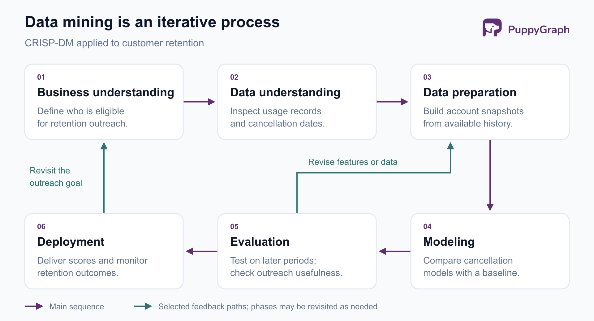
A useful organizing framework is CRISP-DM, the Cross-Industry Standard Process for Data Mining. Its six phases cover business understanding, data understanding, data preparation, modeling, evaluation, and deployment. The process is iterative: findings in a later phase can send a team back to an earlier one. IBM's CRISP-DM documentation describes these dependencies.

Business understanding. Define the decision the work should improve. For a retention project, specify which customers are eligible for outreach, when the team can contact them, and what outcome would justify the intervention. A vague objective such as understanding customers provides little guidance for choosing data or measuring success.

Data understanding. Examine the available records before choosing a model. Establish what each row represents, how identifiers connect across systems, and when fields become available. For retention analysis, check whether cancellation dates represent the request date or the end of paid service. That difference changes the prediction task.

Data preparation. Build the dataset around the decision point. Resolve duplicates, handle missing fields, reconcile categories, and create relevant features. A customer snapshot used to predict next month's cancellation should contain only information available when that prediction would have been made.

Modeling, evaluation, and deployment turn the prepared dataset into a result the team can use.

Modeling. Start with a baseline that is easy to inspect, then compare suitable alternatives. Write down the feature definitions, training period, algorithm settings, and data exclusions. This makes it possible to distinguish an actual improvement from a change in the experiment.

Evaluation. Check both analytical quality and operational usefulness. A model may rank customers accurately while mostly selecting accounts that cannot receive an offer. Review representative successes and failures with the people who would act on its output.

Deployment. Deliver the result through a workflow: a scheduled score, an investigation queue, a dashboard, or a revised business rule. Assign ownership for monitoring, feedback, and updates. A one-time analysis also needs a clear handoff explaining what decision it supports and where its conclusions stop.

Preparation also requires choosing the unit of analysis. A table with one row per order answers different questions from one row per customer. Joining order rows to multiple support tickets can multiply records and inflate totals unless the aggregation is deliberate. Record these choices alongside feature definitions so that a later refresh preserves the original meaning.

The process should produce an evidence trail as well as a result. Another analyst should be able to identify the source data, reproduce the analysis, and explain why the selected method fits the decision.

What are the main data mining techniques?

The main data mining techniques include classification, clustering, association rule mining, regression, and anomaly detection. They differ primarily in the question they answer and the output they produce.

Classification and regression generally learn from examples with known targets. Clustering and association mining usually explore data without predefined outcome labels. Anomaly detection can use different learning setups depending on whether examples of normal and anomalous behavior are available.

These techniques can work together. A team might cluster accounts for exploration, build a classifier for a defined outcome, and use anomaly detection to review cases outside familiar behavior. Each step still needs its own purpose and evaluation criteria.

Classification in data mining

Classification predicts membership in a predefined category. Examples include whether a message is spam, whether a customer will renew, or which support queue should receive a ticket. Historical examples provide the labels from which the model learns.

Common approaches include decision trees, random forests, and logistic regression. Despite its name, logistic regression is a classification method: it models class probabilities rather than a continuous outcome. The scikit-learn linear-model documentation explains this distinction.

Suppose a support team wants to identify tickets likely to breach a response deadline. Training features might include queue length at arrival, ticket category, and service tier. The outcome must describe the later deadline result. A field written after the breach would give the model information that the live system does not yet have.

Evaluation should reflect the consequences of mistakes. Precision measures the proportion of predicted positive cases that are actually positive. Recall measures the proportion of actual positive cases the model finds. A decision threshold changes which scores become positive predictions, affecting the balance between missed cases and unnecessary interventions. These measures are defined in the scikit-learn model-evaluation guide.

For the support team, that means choosing a threshold that produces a manageable escalation queue while catching enough at-risk tickets. Overall accuracy alone does not establish that the model improves the workflow.

Clustering in data mining

Clustering groups observations by similarity without requiring predefined class labels. It is useful when an analyst wants to explore structure before deciding which categories matter.

K-means assigns observations to a specified number of clusters around centroids. It works best when its distance-based grouping assumptions fit the data. DBSCAN groups dense regions and can mark isolated observations as noise. Hierarchical clustering builds nested groupings that analysts can inspect at different levels. The scikit-learn clustering guide compares these approaches and their assumptions.

A retailer might cluster customers using purchase frequency, average order value, and product-category mix. The resulting groups could suggest different shopping patterns. Names such as frequent replenishment buyers are interpretations added after examining the groups, not meanings supplied by the algorithm.

Feature choices require care. If one numerical feature has a much larger scale than another, it can dominate distance calculations. Including spend in cents alongside purchase counts without considering scaling may group customers mostly by spending. Equally, two customers can appear similar in lifetime totals while having very different recent behavior.

Treat clusters as a working description of the selected data. Check whether they persist across reasonable feature choices and time periods, and whether the distinctions support a real decision. A visually separated plot does not establish that the business has discovered permanent customer types.

Association rule mining

Association rule mining finds combinations of items or attributes that occur together. A rule such as coffee → filters describes how often baskets containing coffee also contain filters. The arrow expresses a conditional association; it does not establish purchase order or causation.

Three measures help interpret a rule. Support is the share of all transactions containing both sides. Confidence is the share of transactions containing the first side that also contain the second. Lift compares that confidence with the overall frequency of the second side. Oracle's association-rule documentation describes the measures.

Consider an illustrative dataset of 1,000 baskets. Coffee appears in 200, filters in 100, and both appear in 60. For coffee → filters:

• Support is 60 / 1,000, or 6%.
• Confidence is 60 / 200, or 30%.
• Lift is 0.30 / 0.10, or 3.

Filters appear three times as frequently among coffee baskets as among all baskets. That could justify testing a recommendation, but it does not show that recommending filters will increase sales. Existing promotions or shelf placement may already explain some of the association.

High confidence can also be misleading when the recommended item is common across almost all baskets. Oracle's explanation of lift illustrates why the baseline frequency matters. Review rule volume, sample size, and commercial relevance before turning a discovered association into an automated recommendation.

Regression in data mining

Regression estimates a numerical outcome, such as delivery duration, demand, or repair cost. It learns from observations with known target values and produces estimates for other observations.

Linear regression models an outcome as a weighted combination of input features. Tree-based regression methods can represent more complex relationships through successive splits of the feature space. The appropriate choice depends on the data and evaluation results, not simply on whether the method can express a more complicated pattern.

For an illustrative delivery estimate, inputs might include route distance, parcel characteristics, and the backlog known at dispatch. Actual delivery duration becomes the training target. Events recorded after dispatch belong outside a model intended to make its prediction at dispatch time.

Mean absolute error expresses average absolute prediction error in the target's units. Root mean squared error places greater weight on larger errors. The scikit-learn regression-metrics documentation details these measures. A logistics team should also inspect whether errors systematically increase for particular routes or service levels.

Time matters when regression supports forecasting. A random split can give an unrealistic evaluation if the deployment task is predicting future periods. Test against later observations, using information that would actually have been available, and compare against a simple baseline such as the previous period's value.

Anomaly detection in data mining

Anomaly detection identifies observations that differ from an expected pattern. It is useful when unusual cases deserve attention but reliable labels are scarce or incomplete.

The reference pattern might be a fleet's operating behavior, an account's transaction history, or the local neighborhood around an observation. Isolation Forest isolates observations through random partitioning; Local Outlier Factor compares local density. The scikit-learn outlier-detection guide also distinguishes detecting outliers in existing data from detecting novel observations against a reference dataset.

Consider a machine whose vibration rises while operating under an otherwise familiar load. A detector could flag that observation for inspection. Comparing vibration across all machines without considering operating conditions might instead flag normal behavior from a different equipment class.

An anomaly score measures departure according to the method's assumptions. It does not establish a failed component, a fraudulent payment, or a security incident. Those conclusions require additional evidence.

Evaluate the resulting review workload as well as the detector. Track which alerts lead to useful findings, which repeatedly reflect harmless operating changes, and which important events were missed. If reviewers cannot work through the queue, raising sensitivity can make the overall process less effective.

Data mining examples

The following examples are illustrative applications to real business workflows, not reports of named companies or measured results. Each shows how the question determines the representation and method.

Finding a product pairing. An online store converts completed orders into baskets of distinct products and mines association rules. A candidate pairing appears promising, but review shows that the products were discounted together during one campaign. The team repeats the analysis outside that campaign before designing a recommendation experiment.

Prioritizing retention outreach. A subscription service builds monthly account snapshots and predicts cancellation in the following month. Recent usage decline and unresolved support issues are candidate features. The team evaluates later months, then tests whether outreach changes retention among eligible customers. Predicting departure and preventing it are separate questions.

Investigating shared infrastructure. A marketplace models accounts, devices, and payout destinations as connected entities. Several otherwise ordinary accounts share a payout destination and reuse devices. The pattern becomes an investigation lead. Review must distinguish coordinated abuse from legitimate shared infrastructure, such as an agency managing multiple storefronts.

Estimating replenishment demand. A distributor models weekly demand by product and location. The analyst checks whether low recorded sales reflect weak demand or an inventory shortage that prevented sales. Without that distinction, the model could recommend less inventory precisely where stockouts concealed unmet demand.

In each example, an algorithm produces a candidate signal. Understanding how the records were generated determines whether that signal supports the proposed action.

Data mining use cases

Businesses apply data mining wherever repeated decisions can benefit from evidence across many observations. The useful starting point is a decision owner and an action that can change an outcome.

Customer operations. Retention teams can prioritize outreach, support teams can route requests, and product teams can examine adoption patterns. Each task needs its own target. A score designed to predict cancellation should not automatically become a ranking of who will respond to a discount.

Retail and merchandising. Association analysis can inform product pairings, while regression can support demand planning. Merchandisers need to account for stock availability, promotions, and margins when turning a pattern into a placement or purchasing decision.

Manufacturing and maintenance. Sensor histories and maintenance records can support anomaly detection or failure prediction. Maintenance teams need enough warning to inspect equipment, obtain parts, and schedule work. A signal that arrives after the intervention window has little operational value even if it identifies failures accurately.

Fraud and security investigations. Classification can rank known risk patterns, while anomaly detection and relationship analysis can surface unfamiliar ones. Shared devices, ownership links, or transaction paths provide context for investigation. A relationship becomes evidence to assess, with timing and legitimate explanations kept visible.

Investigating accounts that share devices or payout destinations requires following relationships across records. PuppyGraph lets teams define a graph schema over existing tables so analysts can examine those connections with openCypher and Gremlin. The graph-modeling documentation explains how tables map to nodes, edges, and properties.

Through the default direct-query path, analysts can investigate these patterns in supported SQL databases, warehouses, or lakes without graph-specific ingestion or a persistent duplicate dataset. The resulting connections can guide case review or supply relationship-based features for a predictive model. Predictive modeling and evaluation remain separate tasks in the analytical workflow.

Benefits of data mining

Data mining can improve how teams allocate attention and test decisions. Those benefits depend on the quality of the evidence and the operational response.

More focused review. Ranking tickets, transactions, or maintenance candidates can direct limited capacity toward cases with stronger signals. Measure the value of completed reviews, not just how many records received a score.

More informative planning. Demand estimates and customer-behavior patterns can help teams examine assumptions behind purchasing, staffing, and outreach. Segment-level results may reveal problems that an overall average conceals.

Repeatable decisions. A documented dataset, model, and evaluation process makes it easier to compare proposed changes. Teams can revisit the same decision criteria as new data arrives instead of relying on an undocumented analysis.

Testable hypotheses. A discovered association can motivate an experiment. For example, a recurring product pairing suggests a recommendation to test, while a support pattern suggests a change in routing. The analysis narrows what to investigate; the test establishes whether the intervention helps.

The measurement window matters too. A retention offer may produce an immediate acceptance without changing whether the customer stays. A maintenance alert may trigger an inspection whose benefit becomes clear only later. Choose an outcome and follow-up period that capture the intended effect, and retain enough context to compare the result with the previous process.

A useful business case connects the analytical output to an action, then measures that action against its cost. Better model scores are intermediate evidence, not the final benefit.

Challenges and limitations of data mining

Data mining can produce plausible results that fail in practice. Several recurring problems deserve attention throughout the project.

Data quality and meaning. Missing values, duplicate identities, inconsistent timestamps, and changing definitions can distort patterns. A blank field may mean unknown, unavailable, or not applicable. Treating those states as interchangeable can erase a distinction the analysis needs.

Leakage and overfitting. Information unavailable at prediction time can make evaluation results look unrealistically strong. Repeatedly adapting a model to the same evaluation data also weakens the independence of that check. Fit preprocessing on training data and preserve a final evaluation set. The scikit-learn common-pitfalls guide explains leakage and how pipelines help prevent it.

Selection effects and causality. Historical records reflect earlier business decisions. Reviewed transactions may be more likely to have confirmed fraud labels, and promoted products may have more sales. A predictive relationship does not establish what would happen if the business changed its policy.

Changing behavior. Customers, equipment, and workflows change. Monitor input distributions, missing fields, predictions, and eventual outcomes. Decide who investigates a deterioration and whether the response is retraining, changing features, or revisiting the original question.

Privacy, access, and operational cost. Combining datasets can expose sensitive relationships that are less apparent in individual records. Limit inputs and outputs to what the task requires, and define access and retention practices. Include data preparation, compute, review effort, and ongoing maintenance when assessing feasibility.

These limitations make ownership essential. Someone must be responsible for the dataset's meaning, the evaluation's credibility, and the decisions made from the output.

Conclusion

Data mining turns recorded observations into patterns, predictions, and investigation leads. Classification, clustering, association rules, regression, and anomaly detection answer different questions, so the choice of technique should follow the decision being made.

Start with a defined outcome, build data that matches the decision point, and evaluate on evidence beyond the original analysis. When relationships carry the signal, include connected entities in that representation rather than relying solely on isolated record attributes.

Try the forever-free PuppyGraph Developer Edition and book a demo with the team to see how openCypher and Gremlin queries explore relationships across warehouse and lakehouse tables, with no graph-specific ETL, to support connected-pattern investigation and feature development.