What Are ML Models? Types, Training & Use Cases

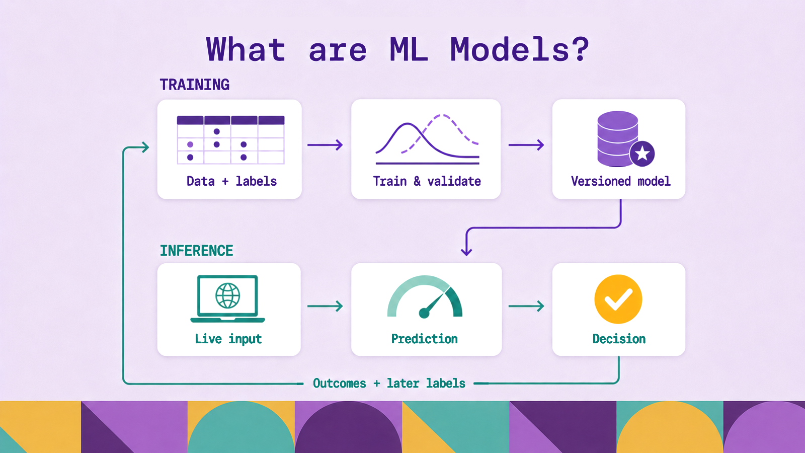
An ML model can score a payment, forecast demand, or generate text, but its result matters only when it improves a real decision. Inputs must reflect the conditions it was trained for, predictions must arrive in time, and the application must handle uncertainty and errors.

The learned artifact is therefore only one component of a working ML system. Data pipelines produce its features, training code fits its parameters, evaluation determines whether it is useful, serving infrastructure makes predictions available, and monitoring tests whether its assumptions still hold. This article follows that lifecycle from the model itself through training, evaluation, deployment, and production operation.

What are ML models?

An ML model is a function whose internal parameters have been adjusted using data. Google's introduction to machine learning describes a model as a mathematical relationship derived from data that a system uses to make predictions. For a house-price model, the inputs might include floor area, location, and age, while the output is an estimated sale price. For an image classifier, the input is a tensor of pixel values and the output is a probability distribution over classes.

Several related terms describe different parts of the system:

Algorithm. The algorithm defines how learning happens. Gradient descent updates parameters to reduce error; a decision-tree algorithm selects feature splits that separate examples. Different training runs can use the same algorithm and produce different models because their data, settings, or random initialization differ.

Parameters. These are values learned during training. A linear model learns a coefficient for each input feature. A neural network can learn many layers of weights and biases.

Hyperparameters. These settings control the training process or model structure but are not learned in the same way. Examples include a tree's maximum depth, a learning rate, or the number of neural-network layers.

Model artifact. This is the serialized output of training: learned parameters plus enough structural and preprocessing information to reproduce predictions. It should remain associated with its code, data version, configuration, and evaluation results.

Using a trained model is called inference. Training may run periodically and consume substantial compute, while inference may need to answer each request within a strict latency budget. That difference shapes the infrastructure used for each stage.

How do ML models work?

An ML model receives numerical representations called features and applies a learned function to them. A linear model combines features using learned coefficients, a decision tree routes an example through learned conditions, and a neural network applies layers of matrix operations and nonlinear transformations. Each aims to capture a pattern that transfers beyond the training examples.

For supervised learning, each training example includes features and a known target, also called a label. The model produces a prediction, and a loss function measures the difference between that prediction and the target. Training repeatedly adjusts the parameters to reduce loss. Google's guide to choosing a loss function explains that the choice determines how heavily training penalizes different errors. For example, mean squared error can train a regression model, while log loss can train a probabilistic classifier.

Reducing training loss is not sufficient. A model can memorize patterns specific to its training examples and fail on new data, a condition called overfitting. A useful model generalizes: it captures a relationship that also holds for unseen examples. Model capacity, regularization, data coverage, and stopping criteria all affect the balance between fitting the training data and generalizing beyond it.

At inference time, the learned parameters remain fixed. The system applies the training-time preprocessing, creates features, runs the model, and converts its output into an action. A classifier might output a fraud probability of 0.82, but application logic decides whether that triggers review, declines a transaction, or adds evidence to another rule.

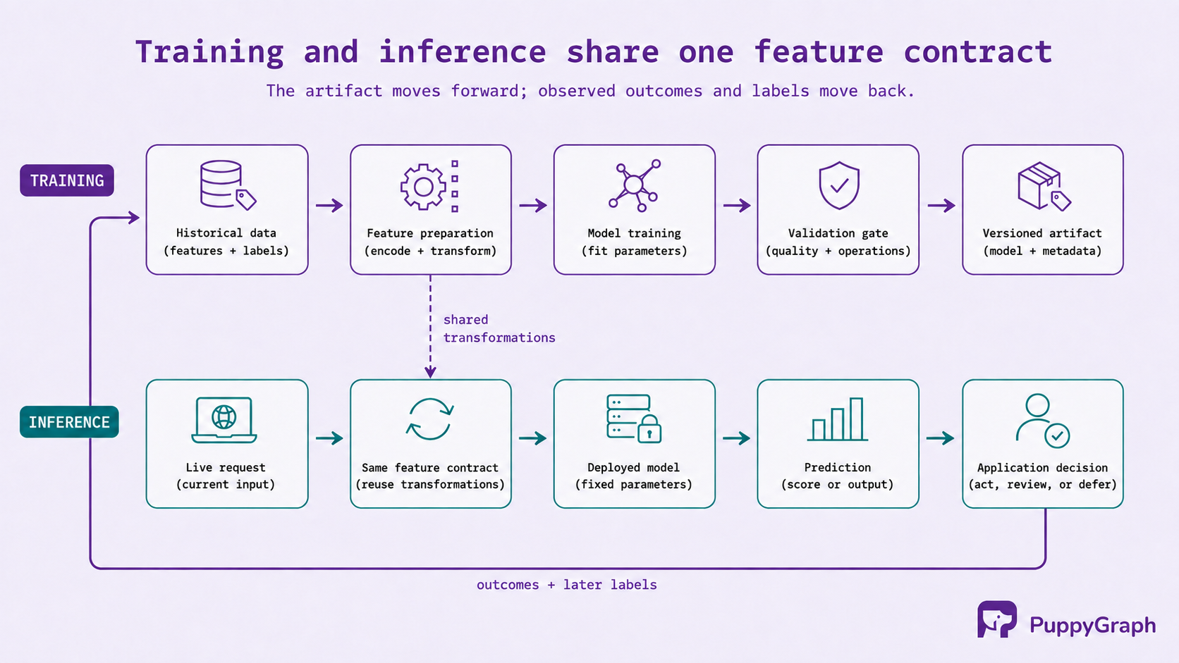
The application decision matters because an ML model estimates or generates; it does not define business policy. Thresholds, fallback behavior, human review, and the cost of different errors belong to the surrounding system.

Types of ML models

ML models can be classified by how they learn and by the mathematical structure they use. These are separate dimensions. Supervised learning is a learning paradigm, while a decision tree is a model family that can be trained within that paradigm.

Supervised learning. A supervised model learns from labeled examples. Regression predicts a continuous value, such as delivery time or energy demand. Classification predicts a category or its probability, such as whether a message is spam. Linear and logistic regression, decision trees, random forests, gradient-boosted trees, support vector machines, and neural networks all support supervised tasks.

Unsupervised learning. An unsupervised model receives data without target labels and finds structure within it. Clustering groups similar examples, dimensionality reduction represents high-dimensional data with fewer variables, and anomaly detection identifies observations that differ from an expected pattern. These outputs still require interpretation. A clustering algorithm can separate customers by behavior, but it does not supply the business meaning of each cluster.

Semi-supervised and self-supervised learning. Semi-supervised methods combine a small labeled set with a larger unlabeled set. Self-supervised methods construct targets from the data itself, such as hiding part of an input and training a model to reconstruct it. This approach underpins many foundation models because unlabeled data is easier to obtain than annotated examples.

Reinforcement learning. A reinforcement learning model learns a policy for choosing actions in an environment. Feedback arrives as rewards or penalties, often after a sequence of decisions rather than immediately after each one. Robotics, game-playing, resource allocation, and some recommendation problems can fit this setup when actions affect future states.

Generative models. Generative models learn enough of a data distribution to produce new samples, such as text, images, audio, or structured records. Large language models, diffusion models, and generative adversarial networks belong here. Generative models can be trained with self-supervision and later adapted with supervised examples or preference-based feedback, so generative describes their output behavior rather than one exclusive training method.

Scikit-learn's user guide illustrates the range within supervised and unsupervised learning, from linear models and ensembles to clustering and matrix factorization. Model selection should start with the task, data, latency, interpretability needs, and cost of errors. A more complex family is useful only when it improves the outcome under those constraints.

How to train an ML model

Training begins before an optimizer touches model parameters. The team must first translate a product or operational objective into a prediction task with a target, available inputs, and a decision that will consume the output. A technically accurate prediction has little value when it arrives too late, depends on information unavailable at inference time, or does not change an action.

Collect and inspect data. Check whether the dataset represents the population the model will encounter. Inspect missing values, duplicates, label quality, class imbalance, time coverage, and sampling bias. Preserve source provenance for reproducibility and debugging.

Prepare features and labels. Convert raw fields into consistent numerical inputs. This can include encoding categories, normalizing values, tokenizing text, aggregating events over time, or calculating relationships among entities. Fit preprocessing transformations only on training data, then apply the fitted transformations to validation, test, and production data. Otherwise, information from evaluation data can leak into training.

Split the data. The training set fits parameters. The validation set supports hyperparameter tuning, threshold selection, and model comparison. The test set provides a final estimate after those choices are complete. Google's guide to training, validation, and test sets emphasizes that evaluation examples must be separate and representative. Random splits work for many independent observations, but time-dependent or grouped data often needs a chronological or group-aware split to prevent future information or related records from crossing the boundary.

Fit, tune, and compare. Start with a simple rule, historical average, majority class, or established model as a baseline, then train candidates and measure them on validation data. The comparison reveals whether added complexity creates material value and can expose misleading results caused by class imbalance or leakage. Adjust features, hyperparameters, regularization, or architecture, and record the data snapshot, code revision, dependencies, random seed, configuration, metrics, and artifact.

Validate the complete pipeline. Re-run preprocessing and inference from raw input, not just from a prepared matrix. Test schemas, missing-data behavior, numerical stability, resource use, and compatibility with the intended serving environment. Evaluate the selected candidate once on the held-out test set, then register it only if it passes predefined quality and operational gates.

Some useful features describe connections rather than individual records: shared devices between accounts, paths through a supply network, or communities in transaction data. PuppyGraph runs openCypher and Gremlin queries against data in SQL databases, data warehouses, and data lakes or lakehouses, with built-in graph algorithms callable from those queries. On the default direct-query path, teams can produce relationship-derived values usable as ML features without building a separate graph-specific ETL pipeline or persistent graph copy. Those feature definitions still need the same versioning, point-in-time correctness, and training-serving consistency as any other transformation.

How to evaluate ML models

Evaluation asks whether a model is good enough for its intended decision, not whether it has one high score. The metric must reflect the error costs and the form of the output.

For regression, mean absolute error is easy to interpret in the target's units, while root mean squared error puts more weight on large misses. For classification, accuracy can obscure performance on an uncommon but important class. Precision measures how often positive predictions are correct; recall measures how many actual positives are found. The F1 score balances the two, while ROC AUC and precision-recall curves evaluate ranking across thresholds. Probability estimates also need calibration when a predicted 20 percent risk is expected to occur about one-fifth of the time.

The scikit-learn metrics guide separates metrics for classification, multilabel ranking, regression, and clustering, and advises choosing a scoring function based on the task and prediction goal. Choose a primary metric before tuning, add guardrail metrics for unacceptable failure modes, and compare all results with a baseline.

Evaluate across relevant slices, such as device type, geography, customer segment, or input quality band. Aggregate performance can hide a severe failure in a smaller group. Use cross-validation when data is limited and observations can be partitioned without leakage. For temporal problems, backtesting across multiple historical cutoffs gives a more realistic view than shuffling past and future records together.

Offline evaluation should also include robustness tests, malformed and missing inputs, threshold sensitivity, latency, memory use, fairness checks appropriate to the use case, and a review of false positives and false negatives. A final test-set score remains an estimate. A staged production release is the next source of evidence.

ML model deployment

Deployment makes a validated model available within a real decision path. Common serving patterns include batch prediction over a scheduled dataset, online inference behind an API, stream processing for events, and on-device inference at the edge. The right pattern follows from how fresh the prediction must be, how much throughput the system handles, and what compute and network access are available.

A deployable unit includes more than model weights. It must reference preprocessing, feature definitions, runtime dependencies, schema contracts, thresholds, and version metadata. The serving path should reproduce training-time transformations to prevent training-serving skew.

Before release, test model quality against the current production version, validate model and infrastructure compatibility, and run end-to-end tests on representative requests. Google's guidance on deployment testing for production ML recommends checking both quality regressions and serving compatibility before traffic reaches a new version.

Use a rollout strategy that limits exposure. Shadow deployment sends live inputs to a candidate without using its outputs. A canary sends a small share of traffic to the candidate. A controlled experiment compares outcomes between versions when the application supports it. Each release needs explicit promotion criteria, an owner, and a rollback path to a known model and feature configuration.

ML model monitoring

Production monitoring covers the service, its inputs, its predictions, and its real-world outcomes. A healthy endpoint can return low-latency predictions from a model that has become wrong.

Service health. Track request rate, error rate, latency percentiles, resource use, dependency failures, and prediction availability. These signals show whether the serving system works as software.

Data quality and skew. Check schemas, missing values, ranges, category frequencies, and feature distributions. Training-serving skew means production features differ from the features the model was trained to expect. Data drift means the input population changes over time. Neither proves that model quality has fallen, but both can invalidate its assumptions.

Prediction behavior. Monitor score distributions, class rates, confidence, and unusual output concentrations by model version and important slice. Sudden changes often indicate upstream problems; slow changes may reflect a shifting population.

Outcome quality. When labels arrive, recompute the evaluation metrics used for release and connect them to business or operational outcomes. Labels may be delayed or incomplete, so teams often use proxy signals such as user corrections, returns, escalations, or manual-review outcomes in the meantime. Google's production monitoring guidance recommends tracking live quality as well as training-serving skew and model age.

Every alert needs an action. The response might investigate an upstream source, fall back to rules, roll back a release, adjust a threshold, collect new labels, or start retraining. Retraining should pass the same validation and deployment gates as the original model. Automating it does not remove the need for evidence that the replacement is safer or more useful.

Monitoring closes the lifecycle. Production outcomes reveal new failure modes, new populations, and stale assumptions. Those observations should become evaluation cases and, where appropriate, new training data for the next version.

Conclusion

An ML model is a learned function inside a larger operational system. Its family and learning paradigm determine what it can represent, but data quality, feature availability, evaluation design, serving constraints, and monitoring determine whether it remains useful. A reliable lifecycle defines the decision first, preserves lineage through training, evaluates against realistic unseen data, releases gradually, and connects production behavior back to the next iteration.

Try the forever-free PuppyGraph Developer Edition and book a demo with the team to see how openCypher and Gremlin queries produce relationship-derived values usable as ML features from warehouse and lakehouse tables, with no graph-specific ETL, while the source data remains in place.