What is an Acquaintance Graph? Structure, Examples, and Applications

In our highly connected era, networks abound, whether social, informational, or technological. From the way people meet, to how messages spread, to how machines communicate, the idea of who is acquainted with whom is central. This is where the concept of the acquaintance graph comes into play: a graph modelling entities and their “acquaintance” ties. By studying acquaintance graphs, we open a window into how relationships, introductions, and indirect connectivity shape complex systems. In what follows we’ll define the concept, delve into its structure and mathematics, look at real-world examples, review applications, compare it with related graph concepts, showcase relevant algorithms, and finally discuss practical challenges.

What is an Acquaintance Graph?

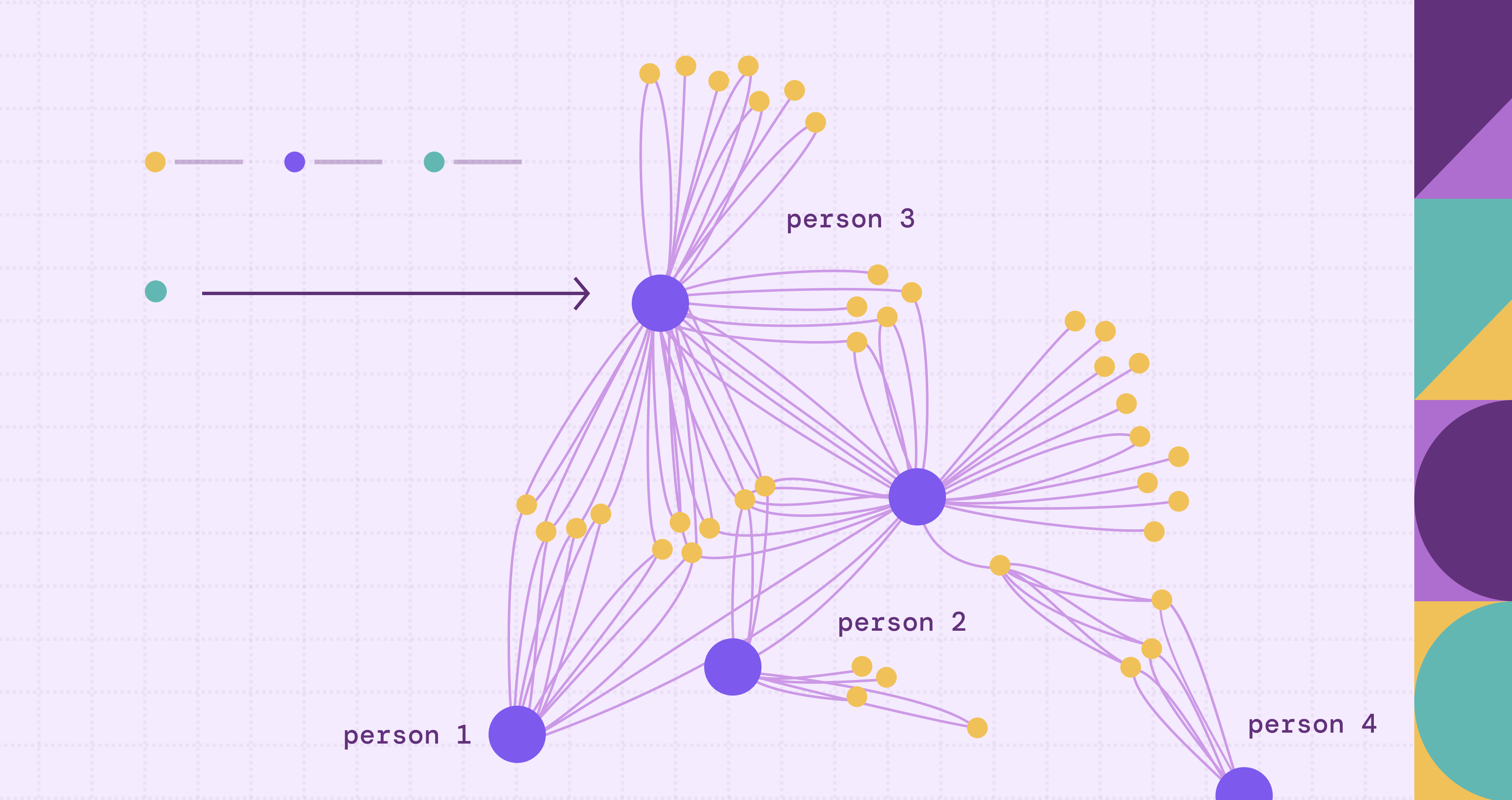
An acquaintance graph is a network model where each node (vertex) represents an entity, typically a person or organization, and each edge (undirected in the simplest form) denotes that the two connected entities are acquainted. That is, there is some form of recognition, familiarity or possible introduction between them. The key idea is that the tie reflects a minimal level of mutual awareness, enough for the two entities to know or introduce each other, even if they are not closely connected.

Definition and Core Concepts

Nodes and Edges

• Nodes represent persons or entities.
• Edges represent an acquaintance relation, usually undirected and unweighted unless otherwise specified.
  In richer models one may attach weights (strength of acquaintance), timestamps (when the acquaintance was formed), or labels (type of tie: professional, personal).

In many treatments, acquaintanceship is symmetric: if A is acquainted with B then B is acquainted with A. Thus, the graph is undirected. (Note: one can generalize to directed or weighted acquaintance graphs when the relation is asymmetric or has strength.)

Why does this matter? Because acquaintance ties often define how networks connect in a “friend-of-a-friend” manner: you may not know someone directly, but you know someone who knows them. That possibility of indirect reach is encoded naturally in acquaintance graphs.

More formally:

Let \(G = (V, E)\) be a graph. Each \(v \in V\) is an entity. Each edge \(\{u, v\} \in E\) means “u is acquainted with v”.

In short: the acquaintance graph models the who-knows-whom backbone of a network, especially when indirect introductions matter.

Variants and Extensions

While the basic form is simple, real‐world acquaintance graphs often include variations that capture richer social or informational nuances:

• Weighted edges: Where the strength or frequency of acquaintance is recorded.
  
  
• Directed edges: If acquaintance is not symmetric (e.g., follower → followed).
  
  
• Temporal dynamics: Edges can form or dissolve over time; modelling this gives a temporal acquaintance graph.
  
  
• Multi‐layer or multiplex graphs: Acquaintance might be one layer (social familiarity) among others (professional ties, online follows).
  
  
• Attributed nodes/edges: Entities (age, location, role) and tie attributes (time of first meeting) enrich analysis.

Structure of an Acquaintance Graph

The structural features of an acquaintance graph mirror many properties of social networks, but with particular emphasis on indirect connectivity, “weak ties”, and introduction paths.

Characteristic Patterns

In acquaintance graphs, you typically encounter:

• Triadic closure: If A knows B and A knows C, then B and C are more likely to know each other. This leads to many triangles in the graph (i.e., high clustering).
  
  
• Short path lengths: Even though you may not know everyone directly, through two or three acquaintance hops you often reach many others (the “six degrees” idea). This is the hallmark of a small-world network. For example, in the small-world phenomenon, the typical distance \(L\) between nodes grows roughly proportional to \(\log N\) where \(N\) is the number of nodes. (Wikipedia)
  
  
• Community and clustering: Groups of nodes densely interconnected (e.g., colleagues, classmates) plus bridges between groups (people who know someone in another group) create modular structure.
  
  
• Bridges and weak ties: According to the sociological insight by Mark Granovetter on The Strength of Weak Ties, acquaintance edges that link distant clusters often enable new information or opportunities to cross communities.

Together, these features explain why acquaintance networks are often both locally dense and globally connected, a defining signature of small-world systems.

Small-world networks and acquaintanceship

Many acquaintance graphs exhibit small-world properties: high clustering and short average path lengths. The small-world concept was formalised by Watts & Strogatz in 1998: networks that combine local groups with global shortcuts. (Wikipedia) Because acquaintance ties often create shortcuts across clusters (friend-of-friend links), acquaintance graphs frequently conform to the small-world paradigm. This property helps explain why information, introductions, or influence can travel so efficiently even in large, seemingly fragmented social systems.

Mathematical Representation

To analyse acquaintance graphs, we invoke standard graph‐theoretic notions, and sometimes specialized ones.

Basic representation

Define \(G = (V, E)\) where \(|V| = n\). The adjacency matrix \(A = [a_{ij}]\) is given by
\[
a_{ij} = \begin{cases}
1 & \text{if } \{v_i, v_j\} \in E,\\
0 & \text{otherwise.}
\end{cases}
\]
The degree of node \(v_i\) is
\[
d(v_i) = \sum_{j=1}^n a_{ij}.
\]

Key metrics

In the context of acquaintance graphs one commonly uses:

• Average degree: This measures how many acquaintances each person has on average. If \( d(v_i) \) is the degree of node \( v_i \) and \( n \) is the total number of nodes, then \(\bar d = \frac1n \sum_i d(v_i)\). It reflects overall network density.
  
  
• Clustering coefficient: It quantifies how likely a person’s acquaintances also know each other. For node \( v_i \), \(C_i = \frac{2E_i}{d(v_i)(d(v_i)-1)},\) where \(E_i\) is the number of links among neighbors. High \(C_i\) implies tight local groups.
  
  
• Average path length and diameter: The average or maximal shortest‐path distances between nodes. Short path lengths are typical in “small‐world” acquaintance networks. (Wikipedia)
  
  
• Connected components: Particularly, whether the network is fully connected (everyone reachable) or splits into disconnected sets.
  

Special concept: Erdős Numbers

A well-known concept illustrating acquaintance distance in collaboration networks is the Erdős number, named after mathematician Paul Erdős. It measures how closely a researcher is connected to Erdős through co-authorship: Erdős himself has number 0, his direct co-authors have 1, their co-authors have 2, and so on. In graph terms, it represents the shortest path length between an author and Erdős in the mathematical collaboration graph, where nodes are researchers and edges represent joint papers.

This idea captures how vast academic communities remain tightly linked through a few acquaintance-like connections, a clear example of the small-world phenomenon. Most mathematicians have an Erdős number below 8, showing the surprising connectivity of the field (source). Similar metrics, like the Bacon number in film networks, generalize this notion to other domains, demonstrating how collaborative ties mirror acquaintance paths in broader social graphs.

Real-World Examples

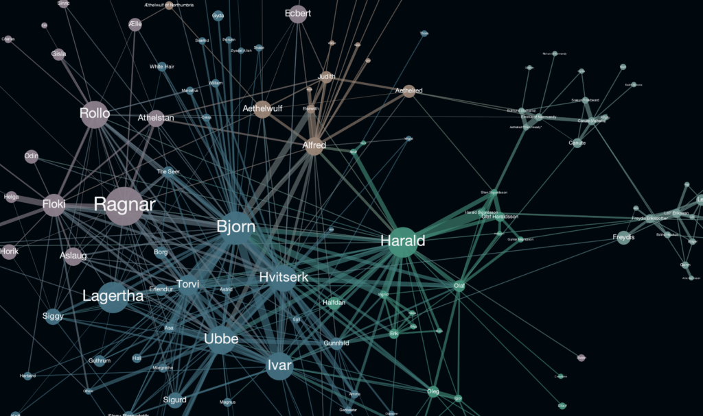
To ground the concept of acquaintance graphs, let’s consider two representative real-world contexts that vividly show how “who knows whom” shapes connectivity and reach.

1. The Six Degrees of Separation phenomenon
   The famous idea of Six Degrees of Separation proposes that any two people on Earth are connected by at most six acquaintance links. In graph terms, it suggests that the average path length between two nodes in the global human acquaintance graph is remarkably short. Originating from social experiments by Stanley Milgram in the 1960s and later confirmed through digital data (e.g., Facebook studies showing an average separation of about 4.5), this illustrates the small-world property: high clustering with short path lengths.
   In practice, this means that even weak acquaintance ties, someone you met briefly or a friend-of-a-friend, can serve as powerful connectors across the network. The “six degrees” idea captures the essence of how acquaintance graphs enable global reach through local links, revealing that the world is far more tightly knit than intuition suggests.
   
   
2. Organisational and online networks
   Within companies or online platforms like LinkedIn, acquaintance graphs expose the informal fabric connecting individuals. Employees who have met across projects or at conferences form cross-department acquaintance ties that foster collaboration and innovation. Similarly, LinkedIn’s “People You May Know” recommendation feature directly leverages two-hop acquaintance paths; if A knows B and B knows C, then A and C might also be worth connecting.
   Such networks demonstrate how acquaintance graphs can illuminate hidden bridges, information flow, and organisational resilience, making them invaluable tools for understanding both human and digital systems.

These examples highlight that acquaintance graphs are not merely abstract constructs but reflect the real architecture of human connectivity, whether across a company, a platform, or the entire planet.

Applications of Acquaintance Graphs

The acquaintance graph abstraction finds utility across multiple domains. Here are four significant application areas.

Social network analysis and sociology

In sociology, acquaintance graphs provide a basis to explore structural features of society: who is connected, how clusters form, how information or influence travels. They enable identifying central individuals who have many acquaintances (high degree), or bridges who link separate communities (high betweenness). For instance, Granovetter’s “weak‐tie” theory suggests that acquaintance ties linking different social clusters bring novel information and opportunities. Using graph‐based metrics, researchers analyse how acquaintance structure influences job mobility, innovation diffusion and social capital.

Graph databases and network modelling

Graph databases (e.g., Neo4j, TigerGraph) and network analytics platforms increasingly host social network data. In such settings, modelling nodes as people and edges as acquaintance ties lets one execute queries like: “Find all people within two acquaintance hops of user X”, “Find the shortest acquaintance chain between Alice and Bob”, or “Suggest new contacts who are acquaintances‐of‐acquaintances”. The acquaintance graph backbone supports recommendation systems, introduction networks, and exploration of indirect connectivity.

Epidemiology, information and contagion spread

Acquaintance networks serve as models for how diseases, memes, or information spread through populations. If individuals are acquainted, they might meet or transmit signals; if they are only connected via acquaintance‐chains, the spread may still occur but with more hops. Understanding path lengths, cluster structure and bridging ties enables one to estimate how fast a contagion may travel, which clusters act as reservoirs, and where interventions (e.g., immunisation, messaging) would be most effective.

Artificial intelligence and relational learning

Modern AI systems increasingly exploit graph‐structured data (graph neural networks, node embeddings, link prediction). If the data graph represents acquaintance ties, then embeddings capture each entity’s neighbourhood of acquaintances, enabling tasks such as: predicting future acquaintance ties (link prediction), recommending new introductions (friend suggestions), classifying nodes by attribute (is this person a connector?), or detecting communities. In short, the acquaintance graph becomes the input ℛ for representation learning and downstream machine‐learning tasks.

Relationship to Other Graph Concepts

By situating acquaintance graphs among other graph types, it becomes easier to recognise their unique features and when they overlap.

Acquaintance graph vs social graph

A social graph is a broad term for any graph modelling social relations: friendships, kinship, professional ties. An acquaintance graph is a specific subset: edges encode acquaintanceship (often weaker ties) rather than every possible social relation. Thus every acquaintance graph is a social graph, but not vice versa.

Acquaintance graph vs friendship graph

A friendship graph includes stronger, more mutual ties (“friends”). Acquaintance graphs are broader: you might be connected even if you are not friends. Accordingly, acquaintance graphs tend to have more nodes and edges, weaker ties, and more breadth; friendship graphs might emphasise depth.

Acquaintance graph vs collaboration/co-authorship graph

Collaboration graphs (e.g., co-authors on a paper) are structurally similar to acquaintance graphs: nodes = actors, edges = collaborated. The difference is semantic: collaboration implies working together; acquaintance implies familiarity or introduction. Nonetheless, analyses of collaboration graphs often use the same structural toolkit (community detection, centrality, clustering) as acquaintance graphs.

Algorithms and Analysis Techniques

When analysing acquaintance graphs we can borrow algorithms from graph theory and network science and adapt them to the acquaintance context. Below are key techniques with focused discussion.

Shortest‐path and reachability analysis

Querying how many acquaintance hops separate two entities, or computing the diameter of the network, reveals how “connected” the network is indirectly. Breadth-first search (BFS) is standard, and the result gives insight about how readily introductions or information may traverse the network.

Community detection and clustering

Algorithms such as Louvain, Girvan-Newman or spectral methods identify modules: groups of nodes with dense acquaintance ties internally and fewer ties externally. In acquaintance graphs this might correspond to social circles, organisational sub-units, or interest groups.

Centrality measures

Metrics like:

• Degree centrality (nodes with many acquaintances)
• Betweenness centrality (nodes acting as bridges between communities)
• Closeness centrality (nodes minimizing hops to all others)
  Are useful to identify key individuals in an acquaintance network, the connectors, influencers, or brokers.

Link prediction and embedding

Since acquaintance graphs naturally model “who might meet whom”, link prediction algorithms are relevant. Techniques such as Common Neighbours, Adamic/Adar, or machine‐learning using graph embeddings (node2vec, GraphSAGE) estimate the likelihood that two currently unconnected nodes will form an acquaintance.

Example: Python code snippet

Here is a simple example using Python and NetworkX to generate a small‐world style acquaintance graph and compute some metrics:

import networkx as nx

# Generate a Watts-Strogatz small‐world graph (e.g., modelling acquaintance ties)
n = 100      # number of nodes
k = 4        # each node is initially connected to k nearest neighbours
p = 0.1      # rewiring probability (introducing shortcuts)
G = nx.watts_strogatz_graph(n, k, p)

# Compute degree, clustering coefficient, average path length
degrees = dict(G.degree())
avg_degree = sum(degrees.values()) / n
clustering = nx.average_clustering(G)
try:
    avg_path_length = nx.average_shortest_path_length(G)
except nx.NetworkXError:
    avg_path_length = None  # graph may be disconnected

print(f"Avg degree: {avg_degree:.2f}")
print(f"Clustering coefficient: {clustering:.3f}")
if avg_path_length:
    print(f"Avg shortest path length: {avg_path_length:.2f}")

This code demonstrates how acquaintance-style graphs can be generated and analyzed programmatically.
These metrics highlight key structural properties of such networks:

• Average degree:  the typical number of acquaintances per node, reflecting local connectivity.
• Clustering coefficient: the tendency of an individual’s acquaintances to know one another, capturing community or social cohesion.
• Average shortest path length: the mean number of steps connecting any two individuals, indicating how closely connected the entire network is (the hallmark of a small-world structure).

Challenges and Limitations

While acquaintance graphs are conceptually appealing and analytically tractable, they have inherent limitations and practical challenges.

• Ambiguity of “acquaintance”: What counts as an acquaintance? The threshold may vary across studies or contexts (met once vs multiple times). Inconsistent definitions affect comparability of models.
  
  
• Data sparsity and bias: Many acquaintance ties are unrecorded or private; often only strong ties are logged (e.g., in online networks). Consequently, the observed graph may be incomplete or skewed.
  
  
• Temporal dynamics and decay of ties: Acquaintance relationships change over time. A static snapshot may misrepresent the true evolving network. Temporal graph modelling adds complexity.
  
  
• Scale and computation: Real‐world acquaintance graphs (like those of major social platforms) may have millions or billions of nodes. Computing global metrics or embeddings can be resource‐intensive.
  
  
• Interpretation caveats: High degree in an acquaintance graph doesn’t automatically imply influence; context matters. The semantics of ties (who knows whom and how) must be considered.
  
  
• Privacy and ethics: Mapping acquaintance networks often involves personal data and raises concerns around consent, anonymity, and meaningful use.
  

Thus, while acquaintance graphs offer rich modelling possibilities, sound empirical work must account for definition consistency, data quality, temporal change, computational feasibility, and ethical practice.

PuppyGraph: Zero-ETL Acquaintance Graphs Directly on Your Relational Data

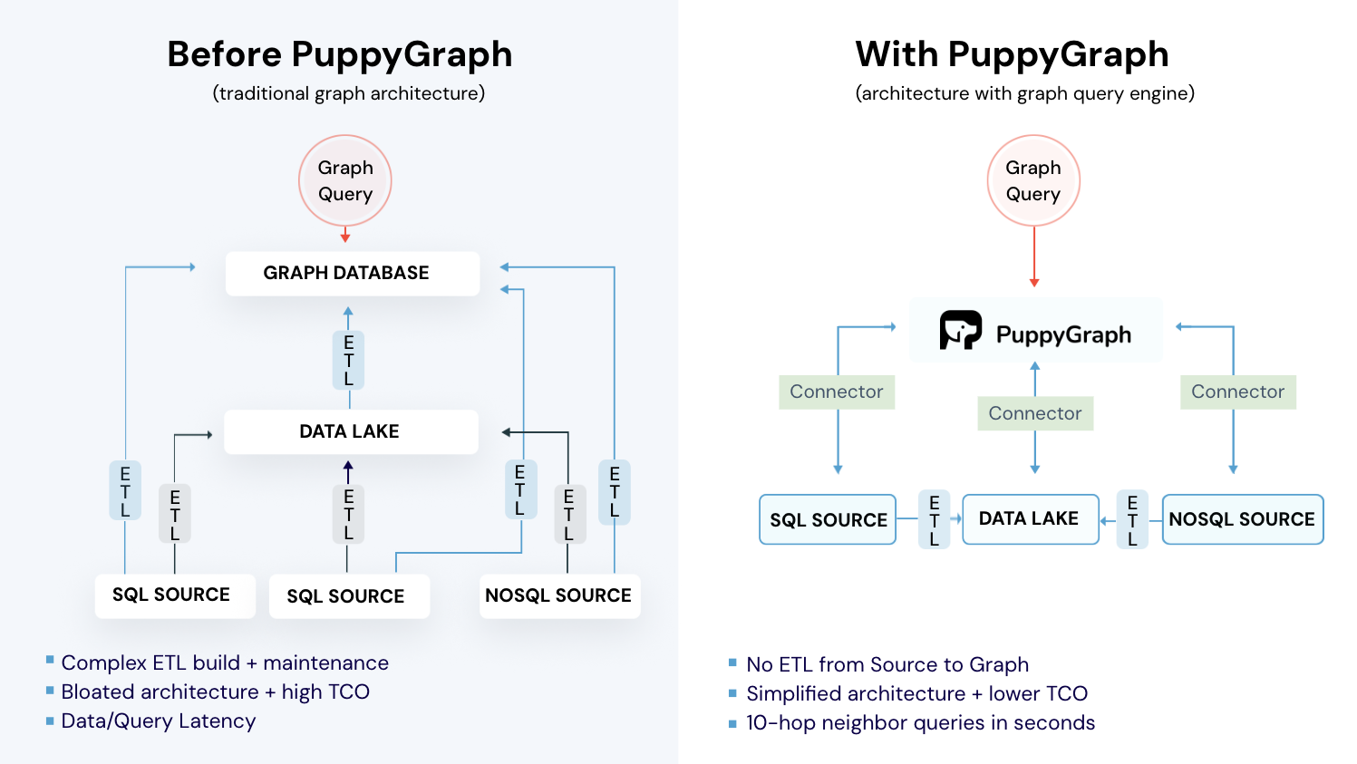
While acquaintance graphs are powerful for modeling “who knows whom”, in practice, building and querying such graphs can be technically daunting. Data lives in relational databases, data lakes, or warehouses, and extracting it into a graph system often means heavy ETL pipelines, data duplication, and maintenance overhead.

PuppyGraph solves this problem with a real-time, zero-ETL graph query engine. It lets teams model and query acquaintance-style graphs directly on top of existing relational and analytical data. Without moving it. In minutes, you can explore how entities connect, how relationships propagate, and how indirect links form, all through expressive graph queries.

Unlike a traditional graph database, PuppyGraph runs as a virtual graph layer. It connects to your data sources (PostgreSQL, Apache Iceberg, Delta Lake, BigQuery, and others) and builds a logical graph view using simple JSON schema files. You can define nodes as entities (like people or organizations) and edges as acquaintance ties, mirroring the same concepts described earlier in this article. Only now, you’re doing it directly on your production data.

Key PuppyGraph capabilities include:

• Zero ETL: PuppyGraph runs as a query engine on your existing relational databases and lakes. Skip pipeline builds, reduce fragility, and start querying as a graph in minutes.

• No Data Duplication: Query your data in place, eliminating the need to copy large datasets into a separate graph database. This ensures data consistency and leverages existing data access controls.

• Real Time Analysis: By querying live source data, analyses reflect the current state of the environment, mitigating the problem of relying on static, potentially outdated graph snapshots. PuppyGraph users report 6-hop queries across billions of edges in less than 3 seconds.

• Scalable Performance: PuppyGraph’s distributed compute engine scales with your cluster size. Run petabyte-scale workloads and deep traversals like 10-hop neighbors, and get answers back in seconds. This exceptional query performance is achieved through the use of parallel processing and vectorized evaluation technology.

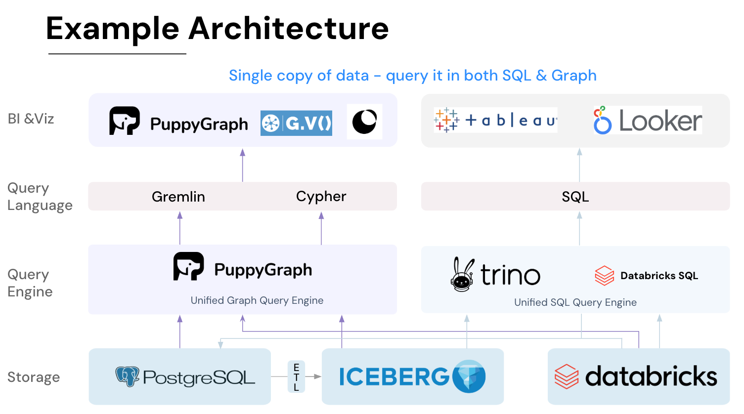
• Best of SQL and Graph: Because PuppyGraph queries your data in place, teams can use their existing SQL engines for tabular workloads and PuppyGraph for relationship-heavy analysis, all on the same source tables. No need to force every use case through a graph database or retrain teams on a new query language.

• Lower Total Cost of Ownership: Graph databases make you pay twice — once for pipelines, duplicated storage, and parallel governance, and again for the high-memory hardware needed to make them fast. PuppyGraph removes both costs by querying your lake directly with zero ETL and no second system to maintain. No massive RAM bills, no duplicated ACLs, and no extra infrastructure to secure.

• Flexible and Iterative Modeling: Using metadata driven schemas allows creating multiple graph views from the same underlying data. Models can be iterated upon quickly without rebuilding data pipelines, supporting agile analysis workflows.

• Standard Querying and Visualization: Support for standard graph query languages (openCypher, Gremlin) and integrated visualization tools helps analysts explore relationships intuitively and effectively.

• Proven at Enterprise Scale: PuppyGraph is already used by half of the top 20 cybersecurity companies, as well as engineering-driven enterprises like AMD and Coinbase. Whether it’s multi-hop security reasoning, asset intelligence, or deep relationship queries across massive datasets, these teams trust PuppyGraph to replace slow ETL pipelines and complex graph stacks with a simpler, faster architecture.

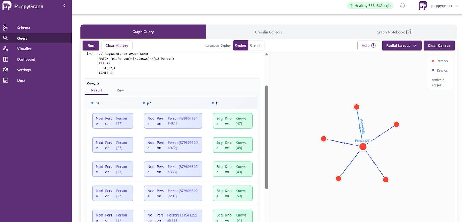
PuppyGraph supports both Gremlin and openCypher, so you can easily express graph patterns like “find all acquaintances within three hops of Alice,” or “discover connectors who bridge otherwise separate communities.” These queries are intuitive in graph form, yet cumbersome in SQL, making PuppyGraph especially suited for acquaintance-graph exploration and relationship analytics.

As data grows more complex, the most valuable insights often lie in how entities relate indirectly. PuppyGraph brings those insights within reach, whether you’re modeling organizational networks, social introductions, fraud and cybersecurity graphs, or GraphRAG pipelines that trace knowledge provenance.

Most teams can start by running PuppyGraph via Docker, AWS AMI, or GCP Marketplace, or deploy it securely inside their VPC for full control. It’s a practical path from acquaintance graph theory to real-world graph analytics.

Conclusion

The acquaintance graph offers a clear yet powerful lens for understanding connectivity in complex systems. By abstracting the idea of “who knows whom,” it captures both direct and indirect ties that drive how information, influence, and opportunities flow. Whether in local communities, organizations, or online networks, acquaintance graphs reveal how small-world patterns, dense clusters linked by a few bridging ties, shape the efficiency and cohesion of social structures.

Mathematically, these graphs rest on well-established principles from graph theory and network science, using measures such as degree, clustering, and path length to quantify structure and reachability. Conceptually, they highlight the importance of weak ties and indirect connections that extend influence beyond immediate neighborhoods. Yet they also require careful interpretation: acquaintance definitions vary, data may be incomplete or dynamic, and relationships evolve over time. Recognizing these nuances ensures that analyses based on acquaintance graphs remain meaningful and contextually grounded.

If you’d like to move from theory to practice, PuppyGraph lets you turn your existing data into a live acquaintance graph instantly. No ETL, no migration, just query. Explore how entities in your systems connect in real time, surface hidden bridges and communities, and unlock graph-level insights across your relational data stack. Download the forever free PuppyGraph Developer Edition, or book a demo with our engineering team.