In large-scale business intelligence, organizations process billions of records from transactions, sensors, applications, and customer interactions. While traditional data warehouse schemas offer structured ways to store and retrieve information, they often struggle under the weight of repetitive, computation-heavy queries. As data volumes grow and analytical expectations rise, maintaining acceptable performance becomes increasingly challenging. This is where the concept of an Aggregate Schema emerges as a powerful optimization technique within dimensional modeling.

An aggregate schema extends a classic warehouse design by adding pre-calculated summaries, or aggregates, that represent rolled-up views of detailed facts. By storing those summaries directly inside the data model, it significantly reduces the query workload on base fact tables. Instead of recalculating totals, averages, counts, or grouped metrics on demand, a query engine can immediately retrieve aggregated data at the perfect level of granularity.

This article explains what an aggregate schema is, how it functions, and why it matters for analytical systems. We explore its structure, operational mechanics, benefits, and limitations, then compare it with the base schemas. Finally, we discuss practical use cases and considerations for implementing aggregate schemas in modern data platforms.

What is an Aggregate Schema?

An Aggregate Schema is an extension of a dimensional data warehouse schema that incorporates summarized or rolled-up versions of fact tables. Instead of storing only the most granular transactional data, the aggregate schema includes tables that represent higher-level summaries, such as monthly totals, weekly counts, or product-category-level metrics. These pre-computed tables act as shortcuts for query engines, enabling faster analytics by reducing the need to process millions of detailed rows during each query.

To illustrate how this works in practice, consider a retail analytics system built on a base schema with product, customer, sales region, and time dimensions, and a transaction-level fact table. The base fact table records individual sales events:

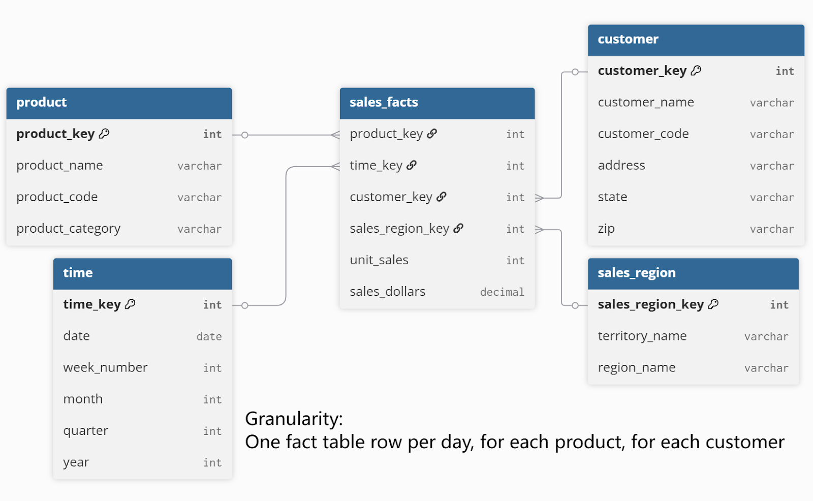
In the base schema example above, the sales_facts table stores the most granular transaction details, capturing every product sold to every customer on each date and in every region. An aggregate schema builds on this foundation by creating summary tables designed to speed up frequent analytical queries.

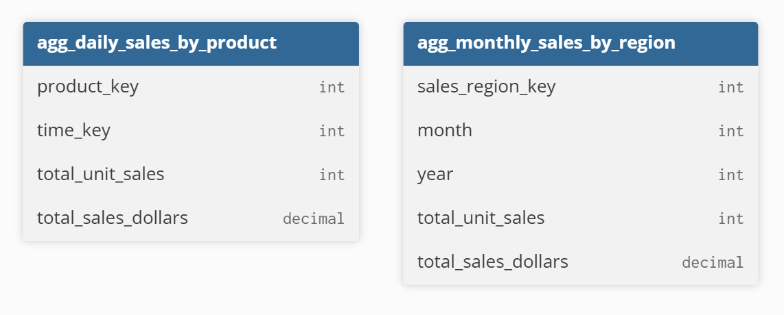
For instance, agg_daily_sales_by_product provides daily sales totals for each product, while agg_monthly_sales_by_region precomputes monthly sales metrics for each region. These aggregates do not replace the original fact table; instead, they serve as a performance layer that reduces the need to scan large volumes of detailed data during analysis.

Aggregates are especially valuable in analytical workloads where users frequently request summarized metrics rather than raw transaction-level details. For example, sales dashboards often show daily revenue, regional comparisons, or trend lines over long historical periods. Without aggregates, each visualization might require expensive scans across large fact tables. The aggregate schema solves this by providing ready-made summaries that dramatically reduce computational costs.

In essence, an aggregate schema is not a different type of warehouse model, but a performance-enhancing layer added to a base schema. It supplements base facts rather than replacing them. The key idea is to pre-calculate metrics that users frequently need and store them in separate fact tables optimized for fast retrieval. This approach improves scalability while preserving accuracy and consistency across analytical queries.

Importance of Aggregate Schemas in Data Modeling

Aggregate schemas play a crucial role in enabling fast and efficient analytics at scale. In many enterprise environments, fact tables grow continuously as new transactions, logs, or events are added. Analytical queries that require joins, grouping, or window functions become slower over time, especially when operating across multiple years of historical data. Without aggregates, systems often attempt to compute summaries repeatedly, overloading compute resources and delaying insights.

One major reason aggregate schemas matter is predictable performance. For instance, in the retail example, computing daily sales for a specific product or monthly revenue by region directly from the sales_facts table would require scanning millions of transaction rows. By using aggregate tables such as agg_daily_sales_by_product or agg_monthly_sales_by_region, queries instead operate on precomputed summaries, reducing the data scanned to just a few thousand rows. This ensures that dashboards load instantly and performance remains consistent, regardless of the underlying data volume.

Aggregate schemas also support analytics teams by enabling more flexible modeling. With summarized data available at multiple granularity levels, analysts can seamlessly explore both detailed insights and high-level trends. Because aggregates are calculated centrally, they maintain governance and consistency while allowing broader access to trusted summaries, enabling teams such as data analysts or sales staff to work with the data safely without needing full access to sensitive transactional details.

Overall, aggregate schemas combine performance improvements with financial and operational benefits, making them an indispensable part of modern data modeling strategies.

Structure of an Aggregate Schema

The structure of an aggregate schema builds on the dimensional modeling foundation established by base schemas. At its core, the aggregate schema keeps the same dimensions, such as product, date, customer, or region, but introduces additional fact tables representing summarized versions of detailed data. These fact tables are derived from the main fact table but contain fewer granularity attributes and fewer rows.

An aggregate fact table typically includes:

1. Foreign keys to dimensions at higher granularity, such as month instead of day.
2. Numeric measures representing totals, averages, counts, or other aggregated calculations.
3. Metadata indicating the aggregation method, time period, or calculation timestamp.

For example, in the previous retail scenario, instead of storing every individual sales transaction from the sales_facts table, an aggregate table like agg_daily_sales_by_product summarizes total quantity and sales per product per day, and agg_monthly_sales_by_region further rolls up sales per region per month.

The dimensions themselves (product, customer, sales region, time) remain unchanged, though sometimes additional “aggregate-friendly” attributes, such as hierarchy levels in the product or time dimensions, are added to facilitate roll-up operations across different granularities.

Because multiple aggregate fact tables may exist within the same schema, their design often depends on expected query patterns. Some warehouses include aggregates at daily, weekly, monthly, and quarterly levels, while others create special-purpose aggregates for high-traffic dashboards.

How Aggregate Schemas Work in Databases

Aggregate schemas rely on a combination of pre-computation, materialization, and intelligent query optimization. The process starts with periodic data processing jobs, often implemented via ETL or ELT pipelines, that read the detailed fact table and calculate summaries at predetermined levels of granularity. These summaries are inserted into aggregate fact tables, which serve as fast-access sources for analytical queries.

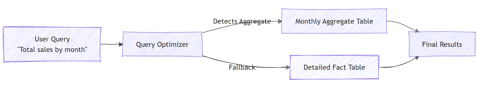
Most modern data warehouses include optimizers capable of detecting when an aggregate table can answer a query. For example, if a user requests monthly sales totals, the query planner may automatically swap the detailed fact table for its monthly aggregate equivalent. This capability is known as aggregate awareness, and systems like Oracle, Snowflake, BigQuery, and SAP BW implement variants of this optimization.

Behind the scenes, aggregate tables reduce computational load by avoiding repeated GROUP BY operations on huge tables. Instead, the heavy computation occurs once during ETL. Some systems also maintain incremental aggregates, recalculating only the portions of data that changed since the last update.

By integrating aggregates directly into the data model, databases achieve near-real-time performance even as data volumes scale. The combination of materialized data and optimizer intelligence makes aggregate schemas a highly effective method for supporting demanding analytics workloads.

Aggregate Schema vs Star Schema vs Snowflake Schema

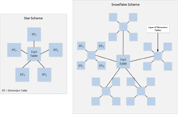
While a star schema organizes data into a central fact table surrounded by denormalized dimensions, and a snowflake schema further normalizes those dimensions into hierarchical tables, an aggregate schema overlays an additional performance strategy on top of either design. The three schemas serve complementary purposes rather than being strict alternatives.

The star schema focuses on simplicity and query efficiency by flattening dimensions. It is easy for analysts to understand, and query engines can join fewer tables. However, star schemas still store only detailed facts, meaning large queries may be expensive to compute repeatedly.

The snowflake schema introduces normalized dimensions to reduce redundancy and improve data governance. While it saves storage space and supports more complex hierarchies, the additional joins sometimes slow down queries. Yet, like star schemas, snowflake schemas alone do not solve performance issues for aggregate-heavy workloads.

The aggregate schema addresses the performance limitations of both by introducing summarized fact tables. These aggregates reduce the need for repeated computation and limit the amount of data scanned. Rather than replacing star or snowflake designs, the aggregate schema enhances them by adding new layers of pre-calculated information.

Together, these schemas represent a range of strategies for balancing ease of use, storage efficiency, governance, and performance. An effective data warehouse often combines all three to achieve optimal results.

Benefits of Using Aggregate Schemas for Analytics

The primary benefit of aggregate schemas is performance improvement. By significantly reducing the number of rows that analytical queries must process, aggregate tables deliver faster results and smoother user experiences, especially for dashboards and BI tools. In cloud-based systems where computation drives cost, aggregates can also lower expenses by reducing the frequency of expensive full-table scans.

Aggregate schemas also enhance business agility by enabling controlled access to data at different levels of granularity. High-level aggregates can be shared with broader teams or executives, while detailed transactional aggregates are restricted to analysts or operational staff. This approach allows organizations to deliver the right information to the right people quickly, supporting faster, informed decisions without compromising data governance. By centralizing the creation of aggregates, teams can confidently use trusted summaries appropriate to their role, ensuring both security and efficiency in data-driven workflows.

Another benefit lies in query simplification. With the right aggregates in place, analysts no longer need to write complex queries with heavy grouping operations. Instead, they can access pre-summarized data that aligns closely with typical analytical needs. This reduces model complexity and helps maintain consistent metrics across teams.

Together, these advantages make aggregate schemas essential for enterprise-grade analytics pipelines that demand speed, consistency, and flexibility.

PuppyGraph Works with Aggregate Tables

If your data sources already include aggregate tables, PuppyGraph can map them directly into graph nodes and edges. This allows graph queries to leverage precomputed summaries for accelerated computation. Instead of repeatedly scanning massive transactional tables, queries can operate on aggregates where appropriate, combining high-level summaries with detailed entity relationships for faster, more efficient analysis.

For example, using the agg_customer_category table, PuppyGraph can create edges from each Customer to their Category with a PURCHASE_SUM property storing the total purchases. A query to find the top categories by total customer purchases could look like this:

MATCH (c:Customer)-[e:PURCHASED]->(cat:Category)
RETURN cat.name, SUM(e.purchase_sum) AS total_purchases
ORDER BY total_purchases DESC
LIMIT 10;

Aggregate tables that summarize data over time, such as daily or monthly sales, can be mapped into graph nodes instead. For example, a DailySales aggregate table can become a node representing a day, with related entity nodes like Customer or Product connected to it via edges. Graph queries can then combine entity relationships with time-based aggregates efficiently.

For instance, to compute total monthly sales for all customers using a time-aggregated node:

MATCH (c:Customer)-[:HAS_DAILY_SALES]->(s:DailySales)
WHERE s.month = '2025-12'
RETURN c.name, SUM(s.amount) AS total_sales
ORDER BY total_sales DESC;

By mapping aggregates into edges or nodes as appropriate, PuppyGraph enables graph queries to fully leverage precomputed summaries, accelerating analysis while preserving detailed relationships and avoiding ETL or data duplication.

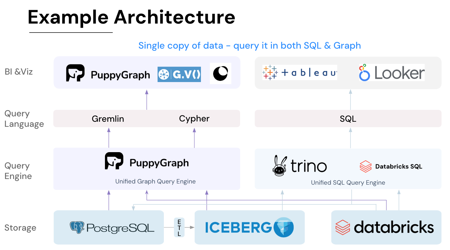
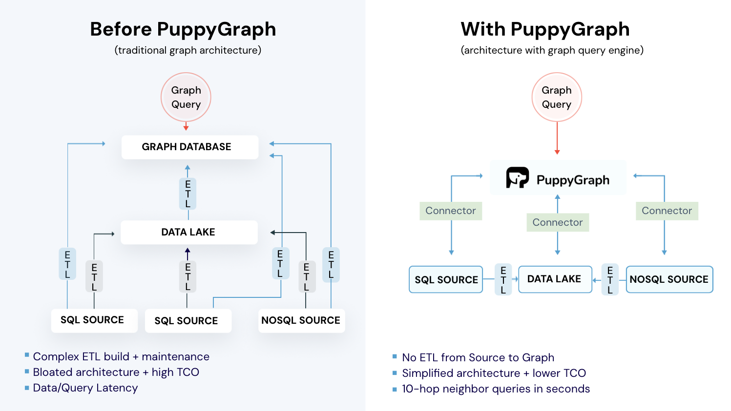
PuppyGraph is the first and only real time, zero-ETL graph query engine in the market, empowering data teams to query existing relational data stores as a unified graph model that can be deployed in under 10 minutes, bypassing traditional graph databases' cost, latency, and maintenance hurdles.

It seamlessly integrates with data lakes like Apache Iceberg, Apache Hudi, and Delta Lake, as well as databases including MySQL, PostgreSQL, and DuckDB, so you can query across multiple sources simultaneously.

Key PuppyGraph capabilities include:

• Zero ETL: PuppyGraph runs as a query engine on your existing relational databases and lakes. Skip pipeline builds, reduce fragility, and start querying as a graph in minutes.

• No Data Duplication: Query your data in place, eliminating the need to copy large datasets into a separate graph database. This ensures data consistency and leverages existing data access controls.

• Real Time Analysis: By querying live source data, analyses reflect the current state of the environment, mitigating the problem of relying on static, potentially outdated graph snapshots. PuppyGraph users report 6-hop queries across billions of edges in less than 3 seconds.

• Scalable Performance: PuppyGraph’s distributed compute engine scales with your cluster size. Run petabyte-scale workloads and deep traversals like 10-hop neighbors, and get answers back in seconds. This exceptional query performance is achieved through the use of parallel processing and vectorized evaluation technology. 

• Best of SQL and Graph: Because PuppyGraph queries your data in place, teams can use their existing SQL engines for tabular workloads and PuppyGraph for relationship-heavy analysis, all on the same source tables. No need to force every use case through a graph database or retrain teams on a new query language.

• Lower Total Cost of Ownership: Graph databases make you pay twice — once for pipelines, duplicated storage, and parallel governance, and again for the high-memory hardware needed to make them fast. PuppyGraph removes both costs by querying your lake directly with zero ETL and no second system to maintain. No massive RAM bills, no duplicated ACLs, and no extra infrastructure to secure.

• Flexible and Iterative Modeling: Using metadata driven schemas allows creating multiple graph views from the same underlying data. Models can be iterated upon quickly without rebuilding data pipelines, supporting agile analysis workflows.

• Standard Querying and Visualization: Support for standard graph query languages (openCypher, Gremlin) and integrated visualization tools helps analysts explore relationships intuitively and effectively.

• Proven at Enterprise Scale: PuppyGraph is already used by half of the top 20 cybersecurity companies, as well as engineering-driven enterprises like AMD and Coinbase. Whether it’s multi-hop security reasoning, asset intelligence, or deep relationship queries across massive datasets, these teams trust PuppyGraph to replace slow ETL pipelines and complex graph stacks with a simpler, faster architecture.

As data grows more complex, the most valuable insights often lie in how entities relate. PuppyGraph brings those insights to the surface, whether you’re modeling organizational networks, social introductions, fraud and cybersecurity graphs, or GraphRAG pipelines that trace knowledge provenance.

Deployment is simple: download the free Docker image, connect PuppyGraph to your existing data stores, define graph schemas, and start querying. PuppyGraph can be deployed via Docker, AWS AMI, GCP Marketplace, or within a VPC or data center for full data control.

Conclusion

In this article we’ve shown how aggregate schemas speed analytics by precomputing summaries and avoiding heavy scans on huge fact tables. They keep performance predictable as data grows while still supporting both detailed and high-level analysis, and they complement base schemas by adding a lightweight performance layer. They also strengthen governance by allowing teams to share high-level aggregates broadly while keeping sensitive transactional data tightly controlled. PuppyGraph maps these aggregate tables into graph nodes and edges so queries use precomputed metrics instead of repeatedly scanning transactions, cutting traversal work and compute time for multi-hop analyses.

Explore the forever-free PuppyGraph Developer Edition or book a demo to see how using aggregate tables to accelerate graph query computation can turn your data into fast, actionable insights.