Arangodb vs Janusgraph : Know The Difference

Graph databases are designed to make connected data and the relationships they represent computable. But depending on your priorities, speed, flexibility, or scalability, the right tool can look very different. It’s impractical to evaluate just featuresets when making a choice; the more important dimensions are data models and infrastructure interactions at scale.

This article compares ArangoDB and JanusGraph, two established yet distinct graph systems. We’ll explore their architectures, query models, performance profiles, and management overhead. We will also highlight the practical trade-offs that matter most in real deployments, and when an alternative like PuppyGraph might provide the balance between simplicity and scale.

What is ArangoDB?

ArangoDB is a distributed, multi-model database that unifies document, graph, and key-value data under a single engine and query language. So you can represent complex, interconnected data structures without deploying multiple specialized databases.

Contrary to some systems that trade flexibility for specialization, ArangoDB’s design leans into generalization as a performance feature; you have one storage engine, one query planner, and one optimizer for multiple data models.

Architecture Overview

ArangoDB uses a shared-nothing clustered architecture that consists of these three components:

• Coordinators: Stateless nodes that handle incoming client queries, decompose them into execution plans, and distribute workloads across data shards.
• DB-Servers: Nodes responsible for hosting the actual data shards and executing query fragments.
• Agents: A consensus layer based on the Raft protocol; it manages cluster configuration, failover coordination, and metadata consistency.

ArangoDB can consequently distribute queries and writes while maintaining predictable performance across replicas. Each collection (ArangoDB’s equivalent of a table) can be automatically sharded based on user-defined keys.

SmartGraphs and Sharding Efficiency

In community editions, graph traversals can span multiple shards, which might cause coordination overhead. To alleviate this, enterprise deployments use SmartGraphs: it guarantees that related vertices and edges reside on the same shard to minimize network hops during traversals. SmartGraphs have impressive performance for large, distributed graph workloads that require real-time responses.

Data and Graph Model

ArangoDB supports three native data models within the same engine:

1. Document model stores JSON-like documents organized into collections.
2. The key-value model is a derivative of documents, accessible through direct key lookups.
3. Graph model defines vertices and edges as documents that support both property graphs and named graphs.

A unified representation means developers can query across these models using a single language, AQL (ArangoDB Query Language), without any necessity to manage separate query engines or ETL pipelines.

AQL and Query Planning

AQL is declarative and composable, supporting nested operations across different models. It combines SQL-like syntax for filtering and aggregation with graph-specific functions like GRAPH_TRAVERSAL, SHORTEST_PATH, and pattern-matching constructs.

For example, the following query finds all vertices connected to Alex within three hops along outbound edges:

FOR v, e IN 1..3 OUTBOUND "users/alex" GRAPH "social"
    RETURN v.name

The query planner automatically determines optimal execution paths across shards and indexes.

AQL’s optimizer is primarily rule-based with cost-based pruning, and it rewrites distributed query plans during compilation to reduce network overhead and improve execution efficiency.

Performance and Storage Engine

ArangoDB uses RocksDB as its underlying storage engine. It is optimized for LSM-tree performance. As a result, you have efficient document and key-value operations even under high write throughput.

Graph performance, however, depends a great deal on data locality. For traversals within a single shard, the performance is near in-memory speeds, while cross-shard traversals incur coordination overhead between DB-Servers.

Query caching and edge index optimizations can substantially improve traversal performance for read-heavy workloads. For Write-heavy deployments, ArangoDB provides configurable write-ahead logs (WAL) for durability and replication safety.

ArangoDB performs best in hybrid workloads. Consider for example, a system that mixes transactional document updates with graph-based recommendation or dependency queries; that makes more sense than ultra-deep traversals spanning billions of edges.

Operational Characteristics

ArangoDB’s distributed architecture emphasizes ease of deployment and predictable failover.

• It achieves high availability (HA) through Raft-based coordination between Agents and replication between DB-Servers.
• Replication is asynchronous by default, with configurable synchronous replication for critical collections.
• The cluster automatically elects new leaders for shards during node failures.
• Backups and Restore is managed through the built-in backup service or ArangoGraph cloud platform.
• In terms of security, ArrangoDB natively supports role-based access control, encrypted communication (TLS), and audit logging.

The open-source edition covers most core features. The Enterprise Edition offers enhancements like SmartGraphs, encrypted backups, LDAP integration, and fine-grained authentication.

What is JanusGraph

JanusGraph is an open-source, distributed graph database built to handle massive graphs that exceed the limits of single-machine systems. It doesn’t maintain its own storage or indexing layer. Rather, JanusGraph functions as a graph processing layer that integrates with proven distributed backends like Apache Cassandra, HBase, ScyllaDB, or Google Bigtable for data storage, and Elasticsearch or Solr for indexing.

This design makes JanusGraph highly modular. It is flexible enough to scale across clusters holding billions of vertices and edges, but dependent on how well-tuned its backend systems are.

Architecture Overview

JanusGraph, being a graph database engine, implements a layered, modular architecture that separates graph logic from persistence and indexing:

• Storage backend: Handles persistence of vertices, edges, and properties. It can be Cassandra, HBase, ScyllaDB, or Bigtable. Each provides fault tolerance, replication, and horizontal scaling.
• Index backend: Enables efficient global searches and lookups. Elasticsearch and Solr are commonly used for full-text and composite indexes.
• Client interfaces: Accessed primarily through the Apache TinkerPop Gremlin API, which serves as both a query language and traversal framework.

Cluster Topology and Data Distribution

Each vertex and edge in JanusGraph is partitioned across nodes based on a hash or vertex ID, with the underlying storage layer handling the replication. This enables linear horizontal scaling, so the graph can grow without centralized bottlenecks.

However, traversal efficiency depends on data locality; queries that stay within the same partition perform faster than those crossing nodes or regions. So to achieve stable performance at scale, you must design an effective vertex partitioning strategy.

Data and Graph Model

JanusGraph implements the property graph model: data is represented as vertices (entities) and edges(relationships), both of which can have key-value properties:

• Directed, labeled edges with arbitrary key-value pairs
• Vertex-centric indexes for efficient edge filtering and property lookups
• Global indexes for cross-vertex queries and analytics

JanusGraph doesn’t enforce rigid schemas; developers can define vertex labels, edge types, and indexes dynamically. 

Query Language and Execution

JanusGraph uses Gremlin, a traversal-based query language from the Apache TinkerPop framework. Gremlin provides a functional, pipeline-like syntax that describes graph traversals as sequences of steps. For example:

g.V().has("user", "name", "Alex").out("follows").values("name")

This query: 

• Starts at vertices labeled user with the property name="Alex"
• Traverses outbound follows edges
• Returns the names of connected users

JanusGraph interprets Gremlin queries and translates them into low-level operations executed across the backend cluster. Traversals that stay local to a partition can execute quickly. Distributed traversals rely on intermediate data exchange between nodes.

Since Gremlin supports both OLTP (real-time queries) and OLAP (batch analytics), JanusGraph can integrate with frameworks like Spark through TinkerPop’s GraphComputer API. 

Performance Characteristics

Traversal Performance

JanusGraph is optimized for wide and deep graph traversals across massive datasets. Its architecture enables scaling to billions of vertices and edges, but with trade-offs:

• Traversals within the same partition achieve near-constant-time performance.
• Cross-partition traversals introduce latency proportional to network hops and storage read consistency levels.

The system’s efficiency heavily depends on backend configuration; Cassandra’s compaction settings, cache hit ratios, and replication factors all impact end-to-end query times.

Write Throughput

Write operations scale almost linearly with cluster size, since data ingestion happens across multiple storage nodes. However, high replication factors and index updates can increase latency. For ingestion-heavy use cases like telemetry graphs or streaming relationships, properly tuned batch mutation strategies significantly improve throughput.

Read Latency

JanusGraph reads rely on backend storage lookups and potential index fetches. As a result, read latency varies between milliseconds to hundreds of milliseconds, depending on the size and locality of the data. Global graph traversals like those touching millions of vertices will benefit from analytical pipelines executed through Spark rather than direct OLTP queries.

Operational and Deployment Considerations

JanusGraph’s flexibility comes with higher operational complexity. Teams must deploy, scale, and maintain multiple components: storage clusters, index backends, Gremlin servers, and client applications.

JanusGraph inherits high availability and replication from the underlying storage backend. Similarly, fault tolerance depends on those layers, not JanusGraph itself.

For monitoring and management:

• Metrics are exposed through Dropwizard or Micrometer integration.
• Clusters can be deployed on-premises or containerized through Docker and Kubernetes, with Helm charts available for orchestration.
• Security features like TLS and authentication depend on the backend systems; JanusGraph itself provides fine-grained access control at the application level.

ArangoDB vs JanusGraph: Feature Comparison

When to Choose ArangoDB vs JanusGraph

When to Choose ArangoDB

Choose ArangoDB when your workloads require multi-model flexibility and predictable query performance under manageable operational complexity.

ArangoDB’s defining advantage lies in its unified architecture: documents, key-values, and graphs coexist in the same query engine, using one optimizer and one transaction model. That makes it ideal for relationship-centric applications but where those relationships don’t dominate; take for example, analytics dashboards, supply-chain systems, or product catalogs. You can correlate structured records and graph relationships without having to maintain separate stores.

JanusGraph offers no native document or key-value model; integrating those requires additional systems, which might escalate the gross complexity. Since ArangoDB offers this natively, data doesn’t have to move among databases, and application logic remains simpler.

When it comes to operations, you can scale and maintain ArangoDB’s self-contained cluster easily. You don’t need to manage distributed storage backends like or index clusters, both of which JanusGraph depends on. That makes ArangoDB a better fit if your team is small, or if you prioritize stability over the ability to scale indefinitely.

Performance-wise, ArangoDB makes for a compelling choice in mid-scale, real-time graphs; there, traversals remain localized and latency matters more. Once graph sizes approach multi-billion edges or traversals become deeply distributed, JanusGraph’s horizontal scale becomes a better choice instead. Until that point, ArangoDB offers the faster and more consistent path to production.

When to Choose JanusGraph

Choose JanusGraph when your data graph is too large for a single engine to handle, or when your organization already operates distributed systems such as Cassandra, ScyllaDB, or HBase.

JanusGraph was designed for distributed, data-intensive environments. It has high modularity, as graph logic is uncoupled from persistence, relying on external systems for storage and indexing. This results in virtually unbounded scaling across nodes and regions, something ArangoDB cannot achieve without hitting vertical limits.

However, this flexibility comes with costs in that you need deep understandings of backend configuration, partitioning, and replication; these particulars are entirely abstracted away in ArangoDB. Evaluate your team’s experience in distributed data operations. Otherwise, you’ll spend more time managing infrastructure than modeling data.

In turn, JanusGraph enables workloads that comprises billions of vertices, multi-terabyte graphs, and streaming or ingestion-heavy systems. ArangoDB can model these scenarios, but it won’t sustain their growth curve without complex sharding strategies and enterprise features like SmartGraphs.

If your environment prefers horizontal elasticity and backend control to simplicity, choose JanusGraph. But if you value coherence, reduced system sprawl, and compact latency control, ArangoDB will deliver faster returns with fewer moving parts.

Which One Is Right for You?

The Argument for ArangoDB

ArangoDB’s integrated model delivers the right balance of power and maintainability for apps that operate within well-balanced boundaries. That means, a few hundred million vertices, localized traversals, and predictable query patterns.

The appeal isn’t necessarily in supporting multiple data models but that those models speak the same internal language. AQL can join documents and traverse relationships in one query plan, with the optimizer balancing cost across collections and graph edges seamlessly.

This design makes ArangoDB a strong fit for mid-scale transactional systems, like recommendation engines, inventory graphs, or internal analytics workloads. The downside is that you get deterministic performance and simple operations, but you inherit the physical limits of a self-contained cluster. Once data distribution or ingestion rate becomes your primary scaling challenge, ArangoDB will need either enterprise extensions or a migration to a more distributed architecture.

The Case for JanusGraph

JanusGraph was designed for environments where the graph spans clusters, regions, or even continents; in such cases, a single node’s memory no longer remains a limiting factor. It extends horizontally by integrating with proven distributed backends, each responsible for persistence, replication, and failover. Teams scale compute, storage, and indexing layers independently, enabling long-term growth beyond the capacity of any single database engine.

However, each of these components must be tuned, monitored, and balanced. For organizations that already operate mature distributed data stacks, this is normal. For smaller teams, it can be overwhelming.

In return, you earn elasticity, fault isolation, and near-unbounded capacity. Massive knowledge graphs, global identity networks, and streaming data relationships are all domains where JanusGraph outperforms any monolithic database. The question is whether your system truly needs that scale today, or whether it’s better served by an engine that minimizes moving parts until scale forces your hand.

Realistically speaking, choose between these systems based not only on graph size, but team maturity and operational context as well. Both make sense, depending on whether you’d rather manage complexity inside the database or across your infrastructure.

Why Consider PuppyGraph as an Alternative

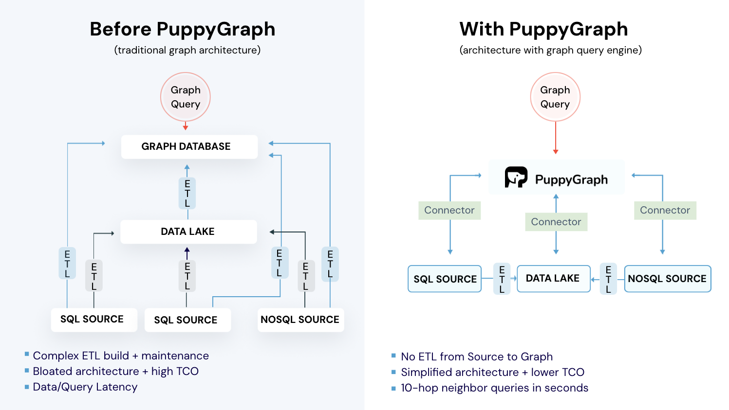
If you’re trying to run graph analytics directly on your existing datasets, both ArangoDB and JanusGraph introduce their own forms of operational drag. ArangoDB requires you to load data into its multi-model engine and maintain a separate copy of your documents and edges, while JanusGraph depends on external storage and indexing systems that must be deployed, synced, and tuned before you can run meaningful traversals. In both cases, you end up managing an additional data system or several just to support graph workloads, which means more pipelines, more storage, and more operational overhead.

PuppyGraph is the first and only real time, zero-ETL graph query engine in the market, empowering data teams to query existing relational data stores as a unified graph model that can be deployed in under 10 minutes, bypassing traditional graph databases' cost, latency, and maintenance hurdles.

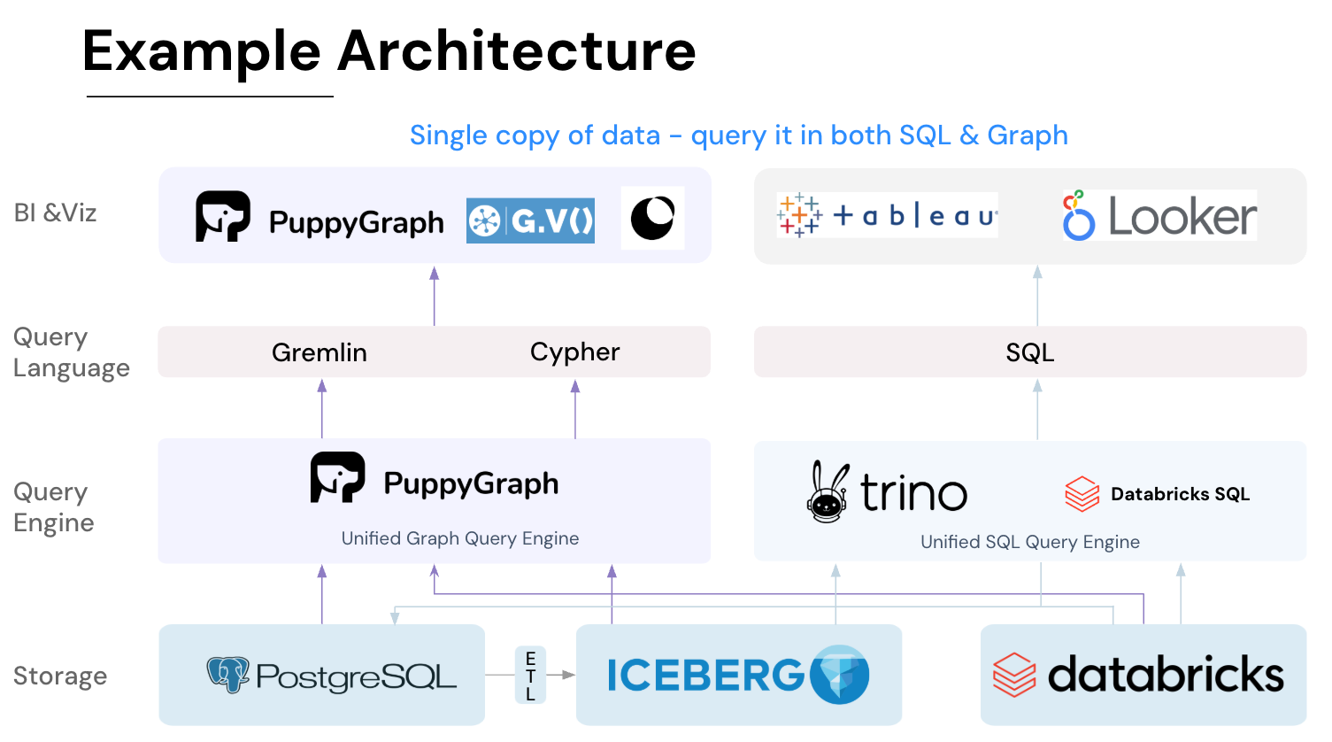
It seamlessly integrates with data lakes like Apache Iceberg, Apache Hudi, and Delta Lake, as well as databases including MySQL, PostgreSQL, and DuckDB, so you can query across multiple sources simultaneously.

Key PuppyGraph capabilities include:

• Zero ETL: PuppyGraph runs as a query engine on your existing relational databases and lakes. Skip pipeline builds, reduce fragility, and start querying as a graph in minutes.

• No Data Duplication: Query your data in place, eliminating the need to copy large datasets into a separate graph database. This ensures data consistency and leverages existing data access controls.

• Real Time Analysis: By querying live source data, analyses reflect the current state of the environment, mitigating the problem of relying on static, potentially outdated graph snapshots. PuppyGraph users report 6-hop queries across billions of edges in less than 3 seconds.

• Scalable Performance: PuppyGraph’s distributed compute engine scales with your cluster size. Run petabyte-scale workloads and deep traversals like 10-hop neighbors, and get answers back in seconds. This exceptional query performance is achieved through the use of parallel processing and vectorized evaluation technology. 

• Best of SQL and Graph: Because PuppyGraph queries your data in place, teams can use their existing SQL engines for tabular workloads and PuppyGraph for relationship-heavy analysis, all on the same source tables. No need to force every use case through a graph database or retrain teams on a new query language.

• Lower Total Cost of Ownership: Graph databases make you pay twice — once for pipelines, duplicated storage, and parallel governance, and again for the high-memory hardware needed to make them fast. PuppyGraph removes both costs by querying your lake directly with zero ETL and no second system to maintain. No massive RAM bills, no duplicated ACLs, and no extra infrastructure to secure.

• Flexible and Iterative Modeling: Using metadata driven schemas allows creating multiple graph views from the same underlying data. Models can be iterated upon quickly without rebuilding data pipelines, supporting agile analysis workflows.

• Standard Querying and Visualization: Support for standard graph query languages (openCypher, Gremlin) and integrated visualization tools helps analysts explore relationships intuitively and effectively.

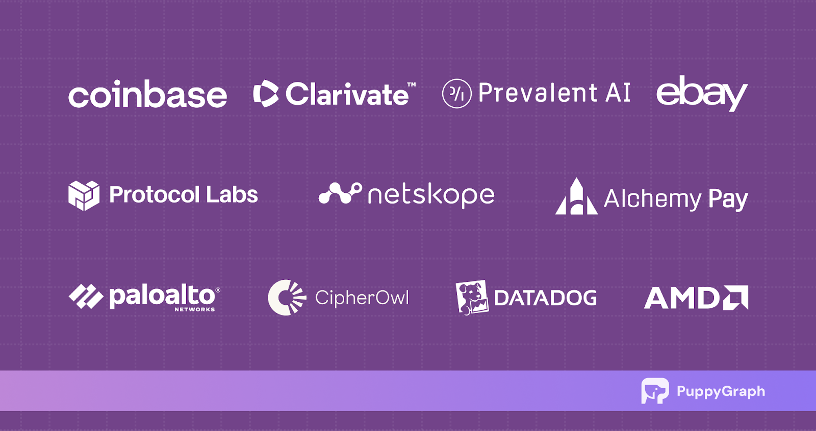
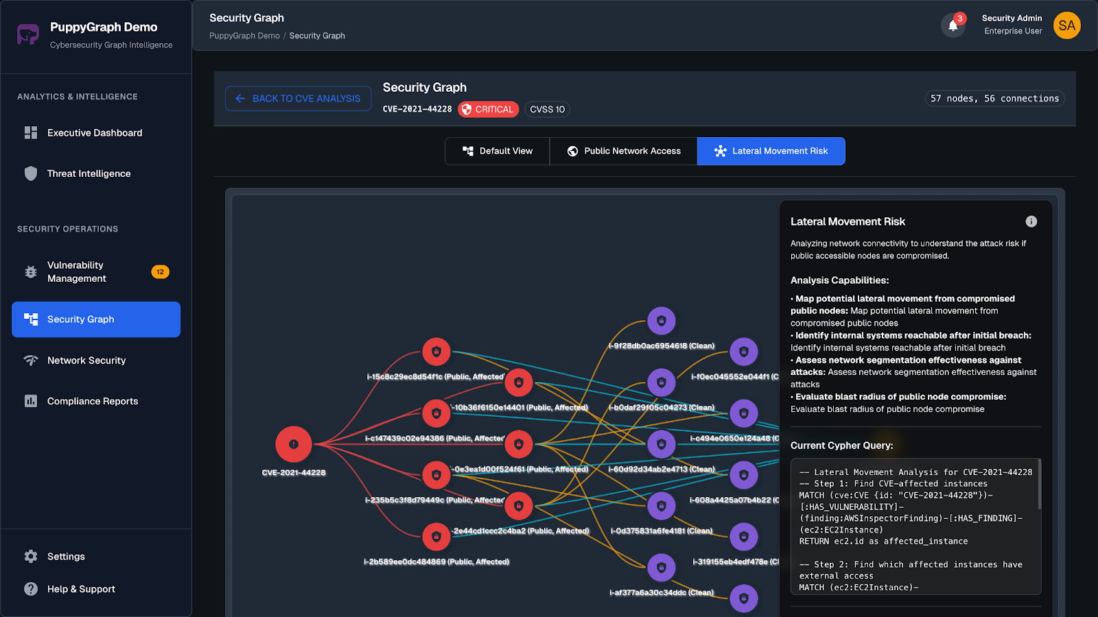
• Proven at Enterprise Scale: PuppyGraph is already used by half of the top 20 cybersecurity companies, as well as engineering-driven enterprises like AMD and Coinbase. Whether it’s multi-hop security reasoning, asset intelligence, or deep relationship queries across massive datasets, these teams trust PuppyGraph to replace slow ETL pipelines and complex graph stacks with a simpler, faster architecture.

As data grows more complex, the most valuable insights often lie in how entities relate. PuppyGraph brings those insights to the surface, whether you’re modeling organizational networks, social introductions, fraud and cybersecurity graphs, or GraphRAG pipelines that trace knowledge provenance.

Deployment is simple: download the free Docker image, connect PuppyGraph to your existing data stores, define graph schemas, and start querying. PuppyGraph can be deployed via Docker, AWS AMI, GCP Marketplace, or within a VPC or data center for full data control.

Conclusion

Modern graph systems have reached a threshold where maintaining separating engines for different workloads is no longer the objective. Rather, it is unifying under one consistent execution model that scales graph-first systems without compromise, sacrificing neither efficiency nor developer ergonomics.

The PuppyGraph platform offers a simple, unified graph engine that does distributed graph computation, with native traversal performance and multi-model flexibility, under one coherent runtime. It eliminates operational trade-offs like ETL, powering real-time analytics, large-scale relationships, and evolving data topologies, all without fragmentation.

To see for yourself how all of this works, get the PuppyGraph's forever free Developer edition, or book a free demo to discuss with our graph experts.