

Backtracking vs DFS: Understanding the Difference and When to Use Each
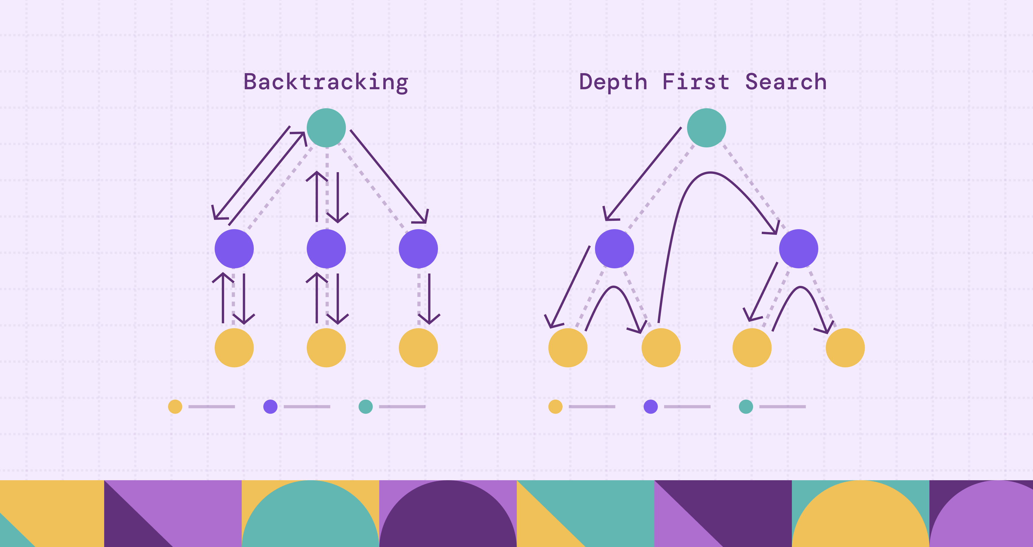
In the world of algorithmic problem-solving, two terms often appear and sometimes cause confusion: Depth-First Search (DFS) and Backtracking. At first glance they seem almost the same: both explore as far as possible down one path then “come back” and try another. But the nuance between them matters. Choosing the right method can mean the difference between an efficient solution and one that runs into combinatorial explosion or misses the right structure for the problem.
In this article we’ll start by clearly defining DFS, then backtracking, then examine how they relate, contrast them in terms of when and how you use them, dive into common misconceptions, explore performance/complexity issues, and finally summarize with guidance for real-world use. By the end you’ll have the vocabulary and the criteria to decide: is this a traversal problem (use DFS), or a search/assignment problem (use backtracking)?
What is Depth-First Search (DFS)?
Depth-First Search (DFS) is a canonical algorithm used to traverse or search within graph or tree data structures. The core idea is simple: from a start node you go as far as you can down one branch before you back up and explore off-shoots. For example, if you're at a root node in a tree, you pick a child and dive; when you hit a leaf or a previously visited node (in a graph) you retreat and then explore the next sibling branch.
In more concrete terms: suppose you have a graph \(G = (V, E)\). You pick a starting node \(v_0\). You mark it visited. Then you pick one of its unvisited neighbours, recurse (or iterate with a stack) to that node. Continue until all reachable nodes from \(v_0\) are visited (or until you find some target). During the recursion you are implicitly maintaining a stack of nodes representing the current path of exploration. When no further move is possible you pop back (return) and try other options. This “go deep then backtrack” pattern is intrinsic to DFS.

Key aspects:
- It is used when you have an explicit structure of nodes/edges (a graph or tree) that you want to explore.
- For a graph of \(|V|\) vertices and \(|E|\) edges (adjacency list), a standard DFS runs in \(O(|V| + |E|)\) time. This is because you visit each vertex and edge at most once (with visited flags).
- DFS uses \(O(|V|)\) space (in the worst case the recursion/stack depth is up to \(|V|\). In trees the depth might be much lower.
- It is often used for connectivity, cycle detection, topological sorting, and other graph/traversal tasks.
- One caveat: DFS does not guarantee the shortest path in an unweighted graph. That’s a property of breadth-first search (BFS).
Thus, when you think of DFS you should picture “visit nodes, go deep, mark visited, back up, explore other branches”.
To make it more intuitive, here’s a simple DFS implementation in Python:
graph = {
    'A': ['B', 'C'],
    'B': ['D', 'E'],
    'C': ['F'],
    'D': [],
    'E': ['F'],
    'F': []
}

visited = set()

def dfs(node):
    if node in visited:
        return
    visited.add(node)
    print(node, end=" ")
    for neighbor in graph[node]:
        dfs(neighbor)

dfs('A')
# Output: A B D E F CWhat is Backtracking?
Backtracking is a more general algorithmic paradigm or technique. Rather than simply traversing an explicit structure, backtracking is often used for searching the space of possible solutions to a problem with constraints. In backtracking you incrementally build a candidate solution, evaluate whether it still can lead to a valid solution, and if not you undo the last step (backtrack) and try a different path.
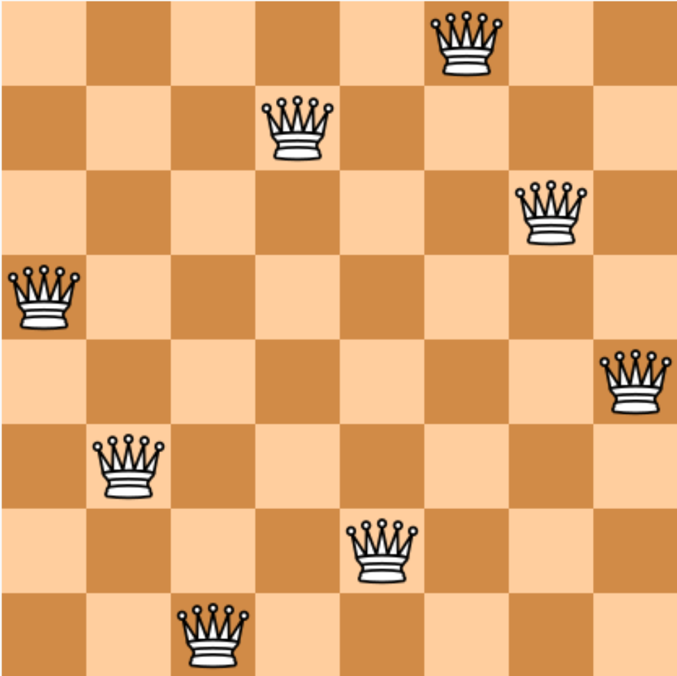
For example, take the classic “N-Queens” puzzle: you place a queen in row 1, then in row 2 you place another in a valid column, etc. At some rows you might discover no valid placement is possible given previous choices, you then backtrack: remove the last queen, move it to the next valid column, and proceed again. That pattern of “choose → recurse → if invalid undo → try next” is what backtracking embodies.
Important features of backtracking include:
- The problem is defined by choices and constraints, rather than an already existing node/edge graph. You are exploring an implicit tree of decision-points.
- You use recursion or a stack to build up a current “partial solution” (or “path of choices”) and at each step you check if the partial solution violates any constraints (if so, you prune).
- You may want all possible solutions, or one solution that satisfies the constraints, not merely traverse a data structure.
- Because the search space is defined by choices, the branching factor may be large and the depth large, so without pruning the time complexity can become exponential.
In summary: backtracking = exploring a search/decision space, maintaining state of partial solution, undoing choices, pruning branches that cannot lead to a valid solution.
Similar to DFS, we provide a sample implementation of backtracking in N-Queens puzzle, to make it easier to understand the concept.
def solve_n_queens(n):
    board = [-1] * n
    solutions = []

    def is_valid(row, col):
        for r in range(row):
            if board[r] == col or abs(board[r] - col) == abs(r - row):
                return False
        return True

    def backtrack(row=0):
        if row == n:
            solutions.append(board[:])
            return
        for col in range(n):
            if is_valid(row, col):
                board[row] = col
                backtrack(row + 1)
                board[row] = -1  # undo choice

    backtrack()
    return solutions

print(len(solve_n_queens(8)))  # Output: 92
Relationship Between DFS and Backtracking
The relationship between DFS and backtracking is subtle: one could say “backtracking uses DFS” or “DFS is a special case of backtracking”. It depends on how you view it. Many sources describe backtracking as essentially DFS applied to the implicit tree of decisions, where you stop exploring certain branches early (prune) based on constraints.
From one viewpoint:
- DFS focuses on traversing a given graph or tree of nodes/edges.
- Backtracking focuses on traversing the search tree of choices (which may be implicit) and uses DFS‐style recursion/stack to do so, but adds the extra dimension of pruning or undoing choices.
For instance, consider a DFS on an explicit graph: you mark visited, you traverse. No explicit “undo choice” is needed beyond retracing recursion. In backtracking, you pick a choice, recurse, then undo/roll‐back the choice and move to the next alternative. The “undo” is central in backtracking.
Another way to look: If you are given a graph and you run DFS, you are exploring all paths (or until you stop) but you are not necessarily evaluating partial solutions or pruning based on constraints. In backtracking, you usually stop exploring a branch before full depth if the partial solution cannot succeed, that is pruning, which is less common (or absent) in plain DFS.
Hence: while they share the “go deep, then retreat” structure, the purpose is different. DFS: traverse nodes/edges. Backtracking: build and test candidate solutions. Recognizing which applies helps significantly when designing algorithms.
Backtracking vs DFS: Key Differences
Below is a table summarizing the key differences between DFS and backtracking:
We can observe from the table that even though their mechanics overlap (both use recursion/stack, both backtrack in some sense), the contexts, goals and constraints distinguish them.
When to Use DFS vs Backtracking
When you face a problem and wonder whether to apply DFS or backtracking, consider the nature of the problem. If you’re given a data structure representing a graph or tree, and you simply need to explore nodes/edges (for example, check connectivity, find reachable nodes, detect cycles), then DFS is the natural choice. It fits directly: pick a start node, mark visited, go deep, back up when needed. Its assumptions and complexity are well understood.
# An example for DFS: a pure DFS traversal on a tree

# Define a simple binary tree node
class Node:
    def __init__(self, val, left=None, right=None):
        self.val = val
        self.left = left
        self.right = right

# Depth-First Search traversal (preorder)
def dfs_tree(node):
    if not node:
        return
    print(node.val, end=" ")  # Visit current node
    dfs_tree(node.left)       # Recurse left
    dfs_tree(node.right)      # Recurse right

# Build a simple binary tree:
#        A
#       / \
#      B   C
#     / \   \
#    D   E   F
root = Node('A',
    left=Node('B',
        left=Node('D'),
        right=Node('E')
    ),
    right=Node('C',
        right=Node('F')
    )
)

# Run DFS traversal
dfs_tree(root)
# Output: A B D E C F
However, if the problem is more like “make a series of choices, subject to constraints, and find one or all valid solutions”, then backtracking is the right paradigm. For example: generate all permutations of a set, solve a logic puzzle (like sudoku) where you place digits under constraints, or combine elements to meet a target condition. In such cases, you are not simply exploring a given graph, you are exploring an implicitly‐defined search space of possibilities. You’ll typically need to prune for efficiency. You’d want to cut off branches that cannot lead to valid solutions early.
# An example for backtracking: generating all permutations of a list

def permute(nums):
    result = []
    def backtrack(path, remaining):
        if not remaining:
            result.append(path)
            return
        for i, num in enumerate(remaining):
            backtrack(path + [num], remaining[:i] + remaining[i+1:])
    backtrack([], nums)
    return result

print(permute([1, 2, 3]))
In some hybrid situations, you might traverse a graph but with constraints (e.g., find a path that meets certain conditions). Then you may embed backtracking logic into a DFS traversal: you explore one path, check constraints, if violated you backtrack immediately rather than finishing exploring. But conceptually you are closer to backtracking because of the constraint‐pruning.
So a quick rule of thumb: if your main goal is “visit/traverse/search the structure”, choose DFS. If your goal is “build/construct solutions from choices under constraints”, choose backtracking.
Common Misconceptions
There are some common misunderstandings around DFS vs backtracking. Let’s clarify a few:
One is the idea that “backtracking and DFS are completely different algorithms.” In reality, backtracking frequently is DFS (or uses a DFS‐style traversal), but with extra logic for state and pruning. As one source succinctly puts it: “Backtracking is a more general purpose algorithm. Depth-First Search is a specific form of backtracking related to searching tree structures.”
Another misconception: “DFS cannot handle constraints, you must use backtracking when constraints are involved.” Actually, you could apply DFS and check constraints in the traversal, but if the problem is fundamentally about exploring decision‐points with undoing, you’re essentially doing backtracking. The difference is more about the problem framing than rigid categories.
There is also a notion that “backtracking is always better because it prunes more.” This is misleading. Backtracking can be more efficient due to pruning, but its worst‐case complexity is still potentially exponential; and if the problem doesn’t require exploring a large search space, DFS might be far more efficient and simpler.
Lastly, many assume “DFS always finds the shortest path.” That is false. Unweighted shortest paths are better found by BFS, not DFS. DFS is not optimal in that sense.
Performance and Complexity
From a performance standpoint, when dealing with an explicit graph with \(|V|\) vertices and \(∣E∣\) edges, a standard DFS will run in \(O(|V| + |E|)\) time, and its space complexity is \(O(|V|)\) (for visited flags and recursion/stack worst-case depth).
In contrast, backtracking explores a decision tree of possible solutions: if at each level there are \(b\) choices (branching factor) and the depth of decisions is \(d\), then in the worst‐case you might explore \(O(b^d)\) candidates (or more). Without effective pruning this leads to combinatorial explosion. With pruning constraints you may reduce the visited space significantly, which is what makes backtracking viable for problems like N-queens, sudoku, etc.
Also, with backtracking, the output size (e.g., number of solutions) may itself be exponential, which means the algorithmic cost is inherently high. On the space side, backtracking typically uses \(O(d)\) space (the recursion depth) plus whatever state is maintained for the partial solutions, which is more manageable than full graph size but still can be large if d is large or state is heavy.
Thus, choosing backtracking demands you are comfortable with potential explosion (unless you can prune aggressively). Meanwhile, for traversal tasks, DFS is predictable and efficient. Recognizing this helps avoid pitfalls: trying to use DFS for a huge combinatorial assignment problem may get you stuck; conversely implementing overly heavy backtracking when a simple DFS would suffice is overkill.
PuppyGraph: Real-Time Graph Queries Without ETL
In the discussion above, both DFS and backtracking revolve around exploring relationships and structures, whether that’s nodes in a graph or choices in a search tree. In the real world, though, your graph often lives inside relational databases and data warehouses, scattered across tables and systems. What if you could apply DFS-like traversal or constraint-based exploration directly on that data, without building a separate graph database?
That’s where PuppyGraph comes in.

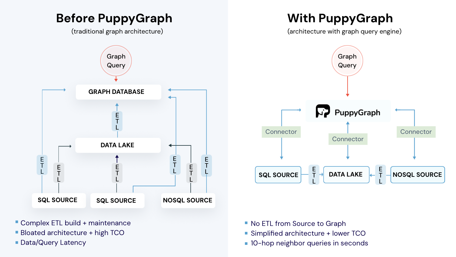
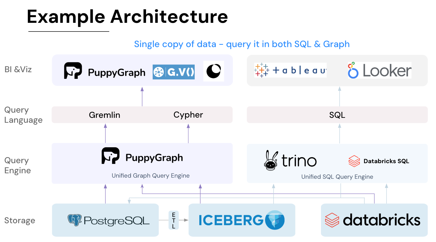
PuppyGraph is a real-time, zero-ETL graph query engine that lets you query your existing relational data as a unified graph instantly. Instead of migrating data into a dedicated graph store, PuppyGraph connects to sources like PostgreSQL, Apache Iceberg, Delta Lake, and BigQuery, then constructs a virtual graph layer on top. You can define nodes and edges using simple JSON schemas and start running graph algorithms in minutes.

Key PuppyGraph capabilities include:
- Zero ETL: PuppyGraph runs as a query engine on your existing relational databases and lakes. Skip pipeline builds, reduce fragility, and start querying as a graph in minutes.
- No Data Duplication: Query your data in place, eliminating the need to copy large datasets into a separate graph database. This ensures data consistency and leverages existing data access controls.
- Real Time Analysis: By querying live source data, analyses reflect the current state of the environment, mitigating the problem of relying on static, potentially outdated graph snapshots. PuppyGraph users report 6-hop queries across billions of edges in less than 3 seconds.
- Scalable Performance: PuppyGraph’s distributed compute engine scales with your cluster size. Run petabyte-scale workloads and deep traversals like 10-hop neighbors, and get answers back in seconds. This exceptional query performance is achieved through the use of parallel processing and vectorized evaluation technology.
- Best of SQL and Graph: Because PuppyGraph queries your data in place, teams can use their existing SQL engines for tabular workloads and PuppyGraph for relationship-heavy analysis, all on the same source tables. No need to force every use case through a graph database or retrain teams on a new query language.
- Lower Total Cost of Ownership: Graph databases make you pay twice — once for pipelines, duplicated storage, and parallel governance, and again for the high-memory hardware needed to make them fast. PuppyGraph removes both costs by querying your lake directly with zero ETL and no second system to maintain. No massive RAM bills, no duplicated ACLs, and no extra infrastructure to secure.
- Flexible and Iterative Modeling: Using metadata driven schemas allows creating multiple graph views from the same underlying data. Models can be iterated upon quickly without rebuilding data pipelines, supporting agile analysis workflows.
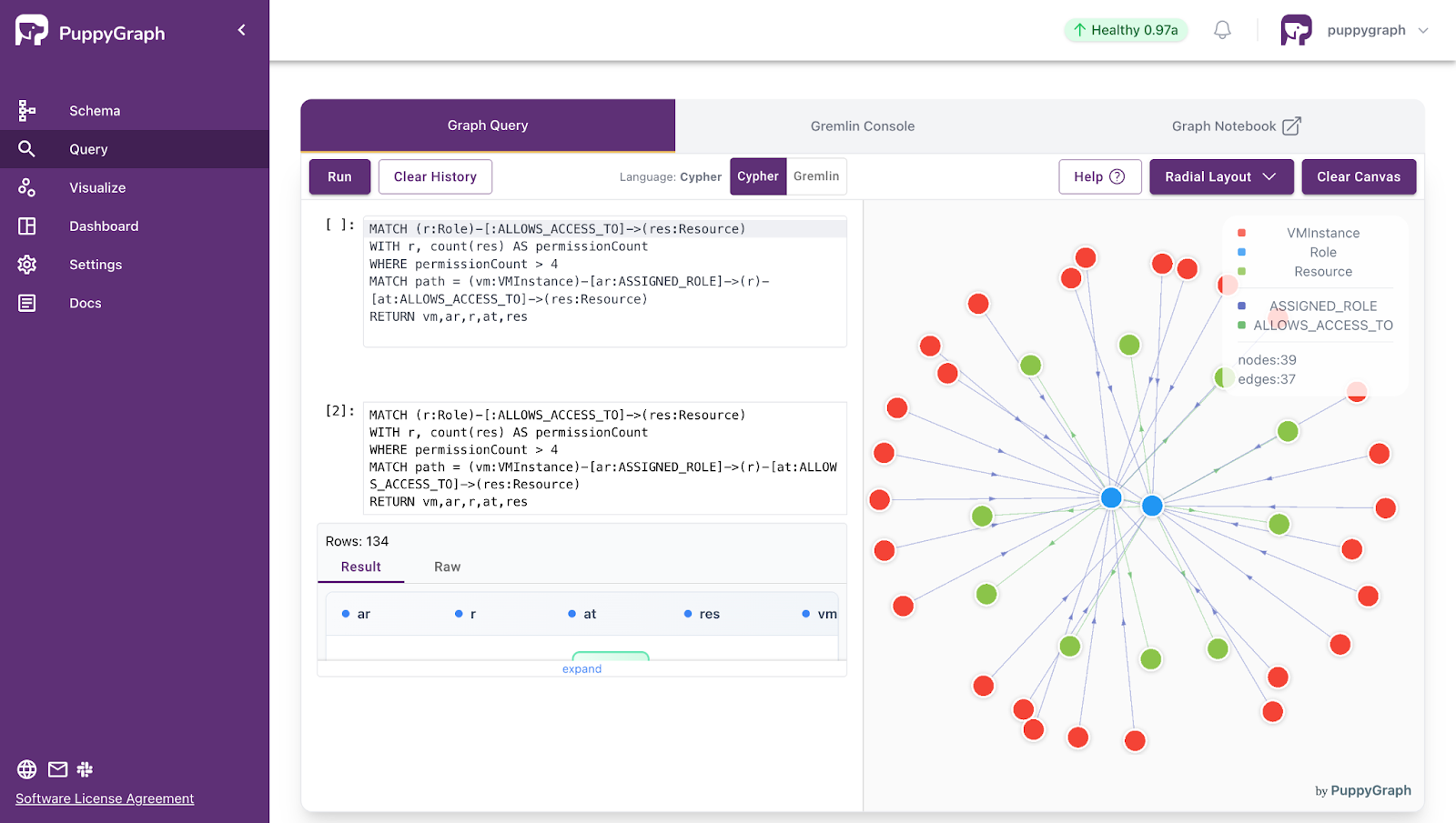
- Standard Querying and Visualization: Support for standard graph query languages (openCypher, Gremlin) and integrated visualization tools helps analysts explore relationships intuitively and effectively.
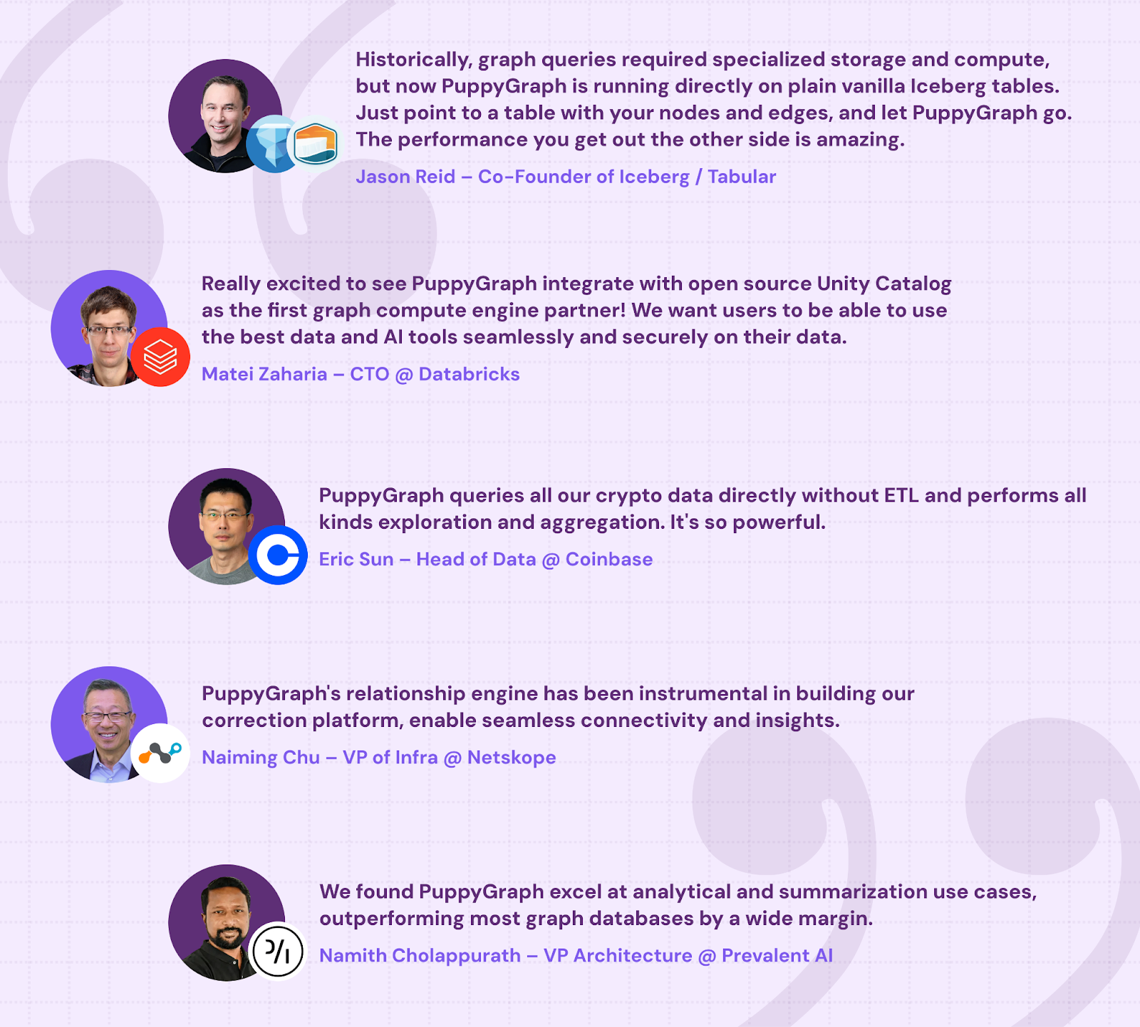
- Proven at Enterprise Scale: PuppyGraph is already used by half of the top 20 cybersecurity companies, as well as engineering-driven enterprises like AMD and Coinbase. Whether it’s multi-hop security reasoning, asset intelligence, or deep relationship queries across massive datasets, these teams trust PuppyGraph to replace slow ETL pipelines and complex graph stacks with a simpler, faster architecture.
As data grows more complex, the most valuable insights often lie in how entities relate. PuppyGraph brings those insights to the surface, whether you’re modeling organizational networks, social introductions, fraud and cybersecurity graphs, or GraphRAG pipelines that trace knowledge provenance.
As data grows more complex, the teams that win ask deeper questions faster. PuppyGraph fits that need. It powers cybersecurity use cases like attack path tracing and lateral movement, observability work like service dependency and blast-radius analysis, fraud scenarios like ring detection and shared-device checks, and GraphRAG pipelines that fetch neighborhoods, citations, and provenance. If you run interactive dashboards or APIs with complex multi-hop queries, PuppyGraph serves results in real time.
Getting started is quick. Most teams go from deploy to query in minutes. You can run PuppyGraph with Docker, AWS AMI, GCP Marketplace, or deploy it inside your VPC for full control.
Conclusion
To wrap up: both DFS and backtracking are fundamental algorithmic ideas you’ll meet frequently. Though their mechanics overlap (recursion, “go deep then retreat”), their use-cases diverge significantly. Use DFS when your job is to traverse or search a defined structure, such as a graph or tree. Use backtracking when your job is to explore a solution space defined by choices and constraints, when you often need to build up partial solutions, test them, undo them, and prune. Recognizing which pattern fits your problem will lead you to better algorithmic choices, efficient solutions, and fewer surprises.
As you face problem after problem, ask yourself: am I navigating nodes and edges, or am I building up candidates and checking constraints? The answer will point you to DFS or backtracking (or sometimes a hybrid). With that clarity, you’ll be more effective in selecting, implementing and optimizing the right algorithm.
With PuppyGraph, DFS, backtracking, or other classic graph traversal methods could be applied directly to your relational tables. You can explore deep connections and run graph algorithms in place without moving or transforming your data. Download the forever-free PuppyGraph Developer Edition, or book a demo to see how it works on your own datasets.

Hao Wu is a Software Engineer with a strong foundation in computer science and algorithms. He earned his Bachelor’s degree in Computer Science from Fudan University and a Master’s degree from George Washington University, where he focused on graph databases.

Get started with PuppyGraph!


Developer Edition
- Forever free
- Single noded
- Designed for proving your ideas
- Available via Docker install
Enterprise Edition
- 30-day free trial with full features
- Everything in developer edition & enterprise features
- Designed for production
- Available via AWS AMI & Docker install