Network analysis has become a foundational technique across disciplines ranging from sociology and epidemiology to cybersecurity and supply chain optimization. At the center of this analytical toolkit lies a family of metrics known as centrality measures, which attempt to quantify the importance or influence of nodes within a network. Among them, betweenness centrality stands out for its focus on control over information flow rather than mere connectivity. Instead of asking how many connections a node has, it asks how often that node acts as a bridge between others.

Betweenness centrality is particularly powerful in identifying brokers, gatekeepers, bottlenecks, and vulnerabilities. It captures the structural position of a node within the larger topology of a graph and helps analysts understand where influence, risk, or leverage may concentrate. In this article, we will examine its definition, mathematical foundation, algorithmic computation, comparison with other centrality metrics, and practical guidance for real-world use.

What Is Betweenness Centrality?

Betweenness centrality is a measure of how frequently a node appears on the shortest paths between pairs of other nodes in a network. In graph theory, networks are modeled as graphs consisting of vertices and edges. If many shortest paths pass through a given node, that node has high betweenness centrality. Conceptually, such a node acts as a bridge that connects different regions of the graph.

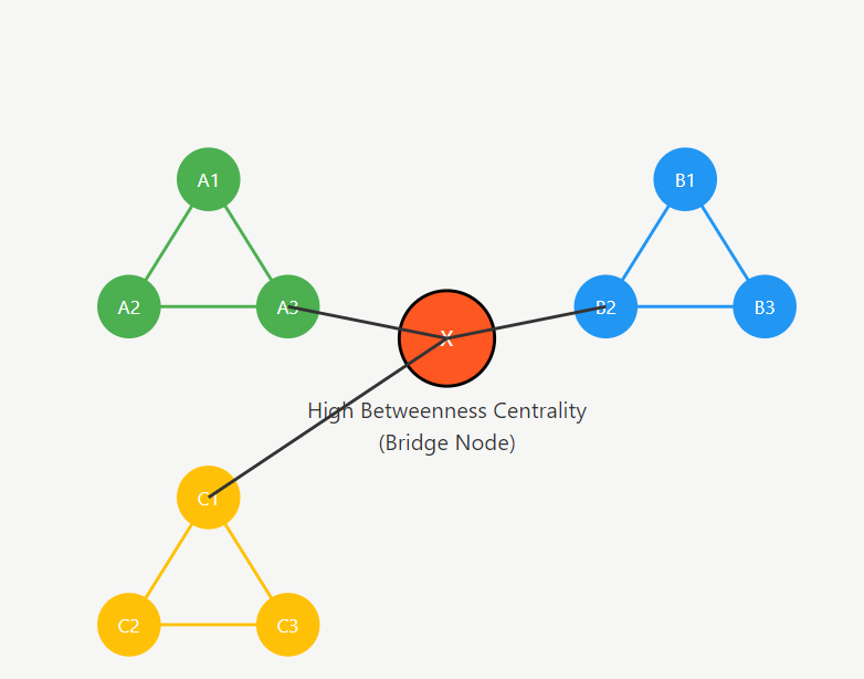
Unlike degree centrality, which only counts immediate neighbors, betweenness centrality captures a more global perspective. A node with relatively few connections can still have high betweenness if it links otherwise disconnected communities. This characteristic makes the metric especially valuable in identifying brokers in social networks or critical routers in communication systems.

The Mathematical Formula for Betweenness Centrality

Formally, the betweenness centrality of a node \( v \) is defined as:

\[
C_B(v) = \sum_{s \neq v \neq t} \frac{\sigma_{st}(v)}{\sigma_{st}}
\]

Here, \( \sigma_{st} \) represents the total number of shortest paths between nodes \( s \) and \( t \), while \( \sigma_{st}(v) \) denotes the number of those paths that pass through node \( v \). The summation runs over all pairs of distinct nodes \( s \) and \( t \), excluding \( v \).

This formula captures the fraction of shortest paths between every pair that are mediated by node \( v \). If a node lies on all shortest paths between many pairs, its score increases significantly. Conversely, if alternative routes bypass the node, its contribution diminishes.

In undirected graphs with \( n \) nodes, normalization is often applied by dividing by \( (n-1)(n-2)/2 \), ensuring the metric ranges between 0 and 1. In directed graphs, the normalization factor is \( (n−1)(n−2) \).  This normalization facilitates comparison across networks of different sizes.

Why Betweenness Centrality Matters in Network Analysis

Betweenness centrality provides insight into the control and mediation roles within a network. Nodes with high values often regulate flows of information, resources, or influence. In organizational networks, such individuals may connect separate departments. In transportation networks, such intersections can represent potential bottlenecks. In communication infrastructures, they may indicate points of vulnerability.

This metric is particularly important because networks are rarely uniform. Many real-world systems exhibit clustering, modularity, or community structure. Betweenness centrality highlights nodes that bridge these clusters, often revealing strategic positions that degree-based measures might overlook.

In epidemiology, nodes with high betweenness can accelerate the spread of disease across communities. In cybersecurity, such nodes may represent critical gateways through which attacks propagate. In supply chain analysis, they may indicate distribution hubs whose disruption would fragment the network.

The broader significance of betweenness centrality lies in its ability to connect structural topology with functional impact. By identifying bridges and chokepoints, analysts can better design interventions, improve robustness, or optimize performance.

Understanding Shortest Paths in Graphs

At the heart of betweenness centrality lies the concept of the shortest path. In graph theory, a shortest path between two nodes is the path with the minimal number of edges, or minimal total weight in weighted graphs. The concept is foundational in algorithms such as Dijkstra’s algorithm and breadth-first search.

Shortest paths represent the most efficient routes for information or resources to travel through a network. Betweenness centrality counts how many of these efficient routes pass through each node. If a node frequently lies along these minimal paths, it effectively mediates interactions between other pairs.

Importantly, multiple shortest paths may exist between two nodes. In such cases, each path is typically counted proportionally. If there are three equally short routes between nodes A and D, and node B appears in only one of them, B receives one-third of the contribution for that pair.

The assumption underlying betweenness centrality is that flows follow shortest paths. While this is a simplifying assumption, it provides a mathematically tractable way to model communication, routing, and influence in many contexts.

Betweenness Centrality in Weighted and Directed Graphs

In practice, many real-world networks are directed and weighted. Financial transactions have direction and volume, communication networks have routing direction and latency, and supply chains encode both flow direction and cost. Therefore, it is most general to treat directed, weighted graphs as the default setting, with undirected or unweighted graphs considered special cases.

A naive algorithm for computing betweenness centrality can be described as follows:

For each pair of nodes \( (s, v) \):

1. Compute shortest paths from the source \( s \):
   Run a single-source shortest-path algorithm (e.g., BFS for unweighted graphs or Dijkstra’s algorithm for weighted graphs) to compute the number of shortest paths from \( s \) to all other nodes.
2. Remove node \( v \) and recompute shortest paths:
   Temporarily remove vertex \( v \) from the graph and run the single-source shortest-path algorithm again from \( s \).
3. Count shortest paths passing through \( v \):
   For each target node \( t \), compare the number of shortest paths before and after removing \( v \).
   The difference gives the number of shortest paths from \( s \) to \( t \) that necessarily pass through \( v \).
4. Accumulate contributions to betweenness:
   Aggregate these values over all targets \( t \) to obtain the contribution of the pair \( (s, v) \) to the betweenness centrality of \( v \).

Since this procedure must be repeated for all pairs \( (s, v) \), the algorithm requires solving the single-source shortest-path problem \( O(n^2) \) times, making it computationally expensive for large graphs.

To address this challenge, Brandes’ algorithm, introduced by Ulrik Brandes in 2001, provides a dramatically more efficient method for computing betweenness centrality. In contrast to the naive approach, Brandes’ algorithm computes shortest-path trees from each source node only once and then reuses these results to accumulate betweenness scores. As a result, it requires only \( O(N) \) single-source shortest path computations (or weighted shortest-path computations using Dijkstra-based variants), significantly improving efficiency compared to recomputing shortest paths for every node pair.

Core Idea of Brandes’ Algorithm

Brandes’ algorithm avoids explicitly enumerating all shortest paths. Instead, it performs a single-source shortest-path computation from each node, while accumulating dependency values that measure how much each node contributes to shortest paths originating from that source.

For a directed, weighted graph, the algorithm proceeds as follows:

1. For each source node \( s \):
   
   • Run Dijkstra’s algorithm to compute:
     
     • The shortest-path distance from \( s \) to all other nodes.
     • The number of shortest paths \( \sigma_{sv} \) to each node \( v \).
     • The predecessor list for each node along shortest paths.
2. Accumulate dependencies (back-propagation phase):
   
   • Process nodes in reverse order of distance from \( s \).
   • For each node \( v \), compute its dependency:
     \[
     \delta_s(v) = \sum_{w: v \in \text{pred}(w)}
     \frac{\sigma_{sv}}{\sigma_{sw}} (1 + \delta_s(w)).
     \]
   • Add \( \delta_s(v) \) to the global betweenness score of \( v \) (excluding the source).

The intuition is elegant: instead of counting paths pair by pair, the algorithm distributes “credit” for shortest paths backward from targets to the source. Each node receives a fraction of dependency proportional to the number of shortest paths that flow through it.

Time Complexity

Brandes’ algorithm reduces complexity substantially. For weighted graphs, the time complexity is \( O(nm + n^2 \log n) \), where Dijkstra with a Fibonacci-heap priority queue is used. For unweighted graphs, shortest paths can be computed using breadth-first search (BFS), reducing complexity to \( O(nm) \).

Betweenness Centrality vs Degree, Closeness, and Eigenvector Centrality

Centrality measures capture different aspects of node importance. Comparing them clarifies the unique contribution of betweenness centrality.

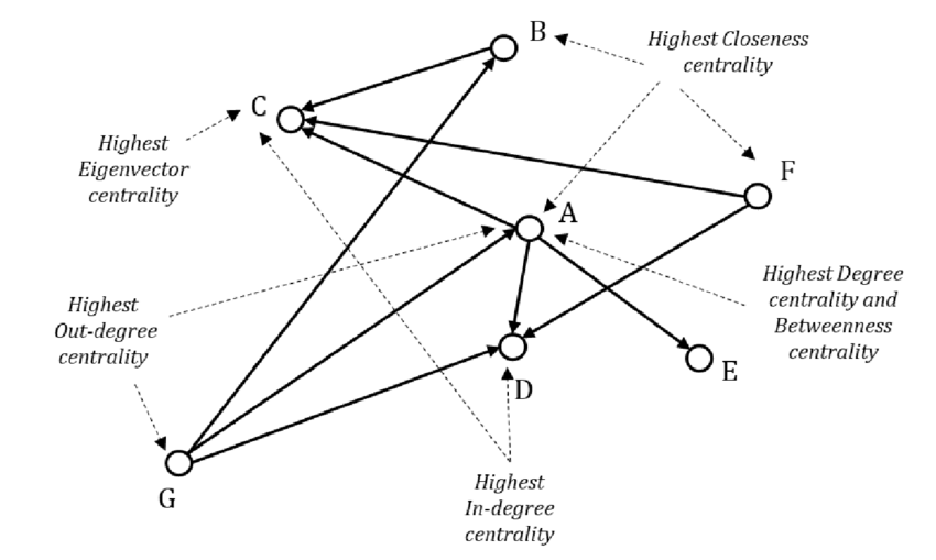
Degree centrality measures the number of immediate neighbors a node has. It is purely local and reflects direct connectivity. A highly connected node may have low betweenness if it does not bridge distinct communities.

Closeness centrality measures how close a node is to all others in terms of shortest path distance. It captures efficiency in reaching others but does not directly measure control over interactions between them.

Eigenvector centrality assigns importance based on connections to other important nodes. It reflects influence within densely connected clusters but may overlook bridging roles between clusters.

Betweenness centrality differs by focusing explicitly on mediation. A node can have modest degree yet possess high betweenness if it connects otherwise separated regions. In community-structured networks, such nodes are often strategically critical.

Choosing among these metrics depends on the research question. If the goal is to find influencers within a cluster, eigenvector centrality may be suitable. If the objective is to detect brokers or vulnerabilities, betweenness centrality is often more appropriate.

Limitations and Interpretation Challenges

Despite its strengths, betweenness centrality has notable limitations. First, it assumes that interactions follow shortest paths, which may not reflect real behavior. In social networks, information may diffuse through redundant or random routes rather than strictly optimal ones.

Second, computation can be expensive for very large networks, particularly weighted or dynamic graphs. Although efficient algorithms exist, scalability remains a concern for networks with millions of nodes.

Third, interpretation can be context-dependent. High betweenness may indicate power and influence, but it can also signal vulnerability. Nodes that serve as bridges may become single points of failure.

Another challenge is sensitivity to small structural changes. Adding or removing a few edges can dramatically alter shortest paths, leading to substantial shifts in centrality values.

Best Practices for Using Betweenness Centrality in Practice

Effective use of betweenness centrality begins with clarity about the research objective. Analysts should verify whether shortest-path mediation aligns with the dynamics of their domain. In transportation or routing contexts, this assumption is often reasonable. In diffusion processes, it may require validation.

Data preprocessing is equally important. Removing noise, handling disconnected components, and ensuring accurate edge weights can significantly affect results. Analysts should also consider normalization to enable meaningful comparisons.

Combining betweenness centrality with community detection methods can provide deeper insight. Identifying clusters first and then examining bridging nodes between them often yields actionable intelligence in organizational or social analysis.

In large-scale systems, approximate algorithms or sampling techniques may be necessary to reduce computational burden. Many graph processing frameworks implement parallelized versions of Brandes’ algorithm to handle industrial-scale data.

Finally, centrality metrics should rarely be used in isolation. Triangulating betweenness with degree, closeness, and domain-specific measures produces more robust interpretations and avoids overreliance on a single structural indicator.

Conclusion

Betweenness centrality is a key metric for understanding how nodes control information flow in a network by measuring how often they appear on shortest paths between other nodes. It helps identify important bridges, brokers, and potential bottlenecks that influence connectivity and robustness of complex systems. While powerful, it should be interpreted carefully due to its reliance on shortest-path assumptions and computational cost in very large graphs.

PuppyGraph provides a practical platform for applying graph analytics at scale by enabling real-time queries directly on existing relational data and data lakes without ETL pipelines. Its zero-ETL architecture, distributed execution, and support for standard graph query languages allow organizations to analyze relationships efficiently while reducing infrastructure complexity and cost.