The relationships between entities seldom remain static. Whether it's social networks evolving as friendships grow or disappear, communication patterns shifting across a fleet of devices, or transactions fluctuating in a financial ecosystem, the underlying structures that capture these interactions are themselves dynamic. A static graph, a fixed set of nodes and edges, often fails to reflect the fluid nature of real-world networks. Enter the concept of a dynamic graph: a powerful abstraction that allows nodes, edges, and even attributes to evolve over time.

In this article, we’ll explore what a dynamic graph is, how it differs from static graphs, the core concepts that underpin them, their varying types, algorithms and data structures tailored for them, methods for visualization, real-world applications (especially in domains such as AI, cybersecurity and data analytics), plus the challenges that arise in dynamic graph analysis. By the end you should have a solid understanding of why and how dynamic graphs matter, what tools and frameworks are used to study them, and where they can really make an impact.

What is a Dynamic Graph?

A dynamic graph (sometimes also called a time-varying graph, temporal network, or evolving graph) refers to a graph whose topology, attributes or node/edge set changes over time. In contrast to a static graph where the nodes and edges are considered fixed for the analysis period, a dynamic graph explicitly models the temporal dimension of evolution: new nodes or edges may appear, existing ones may disappear, and features of nodes or edges may shift.

Formally, one can think of a dynamic graph as a sequence of graph snapshots \(G_{t}\) at different time t, or as a stream of graph events (additions/deletions/updates) annotated with timestamps. For example, one taxonomy defines:

• Discrete-Time Dynamic Graphs where the topology is captured at discrete intervals.
• Continuous-Time Dynamic Graphs where changes are logged as events with exact timestamps rather than discrete snapshots.

This capability to capture evolution makes dynamic graphs a richer and more realistic model for many real-world systems: social networks, mobility networks, communication logs, financial flows, biological networks, and more.

Static vs Dynamic Graphs

To better understand the implications of temporal changes in networks, it is useful to contrast dynamic graphs with their static counterparts.

Core Concepts of Dynamic Graphs

When studying dynamic graphs, several foundational concepts repeatedly emerge. Three in particular: time granularity, temporal evolution, and temporal paths are essential for understanding how networks change over time and why this change matters.

Time Granularity and Representation
Time granularity defines how dynamic graphs capture temporal changes. Snapshot-based methods divide time into intervals, producing static graphs that approximate evolution but may miss interactions between snapshots. Event-based methods record each interaction with exact timestamps, preserving fine-grained activity, bursts, and causal sequences, yet require more storage and computation. Choosing the right granularity balances fidelity and efficiency, ensuring analyses capture meaningful patterns without excessive complexity, making it crucial for understanding network evolution over time.

Temporal Evolution of Nodes, Edges, and Attributes
Dynamic graphs evolve as nodes and edges appear, disappear, or change attributes such as labels, weights, or interaction rates. These changes shape structural patterns, reflecting strengthening or weakening relationships. Attribute shifts often interact with topology, as rising activity reinforces ties while declining engagement weakens them. In domains like finance or communication, evolving weights or risks can reconfigure subgraphs. Tracking these dynamics enables anomaly detection, trend discovery, and more accurate predictions of network behavior over time.

Temporal Paths and Causality
Connectivity in dynamic graphs depends on the timing of edges. Temporal paths follow chronological order, valid only within specific time windows. This time-respecting constraint is essential to trace information diffusion, movement, or transaction sequences accurately. Temporal paths reveal causal chains that static paths cannot capture. Ignoring temporal order can misrepresent reachability, while respecting it ensures analyses reflect real dependencies and the true evolution of the system, allowing correct understanding of influence, flow, and interactions over time.

Types of Dynamic Graphs

Dynamic graphs vary along several axes, how frequently they change, whether changes are discrete or continuous, whether attributes change, etc. Below are common types you’ll encounter.

Discrete-Time Dynamic Graph
Graphs captured at uniform time intervals: \(G_1, G_2, …, G_T\). Each snapshot shows the graph at time-step \(t\). Advantages: easier to manage and compatible with many static graph methods. Disadvantages: may miss events between snapshots.

Continuous-Time Dynamic Graph
Graph changes are recorded as a sequence of events with timestamps, without waiting for uniform intervals. Good for high‐resolution temporal modeling.

Streaming Graph
A subtype of continuous-time dynamic graph often used when data arrive in a stream (e.g., social media interactions, network logs). Algorithms must be capable of online updates, sliding windows, or incremental computation.

Evolving vs Temporal Attribute Graphs
Evolving topology: Nodes/edges added or removed over time.
Attribute dynamics only: Topology remains constant but features/weights on nodes/edges change.
Some systems combine both.

Time-Ordered Multilayer Graphs
In some modeling frameworks, each time slice is a layer in a multilayer graph, with inter‐layer edges representing temporal transitions between time steps. This allows the fusion of temporal and structural analysis.

While the above covers the main types, many real‐world instances are hybrids (e.g., snapshots with attribute changes plus event logs). Recognizing which type your data falls into affects choice of modeling strategy, algorithms, and visualization.

Dynamic Graph Algorithms and Data Structures

Analyzing dynamic graphs demands specialized algorithms and data structures that account for time. Below we highlight key methods and structures, grouped by their primary focus.

Data Structures

Temporal adjacency list / edge lists: Instead of a static adjacency list, you maintain a list of edges annotated with timestamps or time intervals.

Snapshot storage: Maintain a sequence of graph snapshots, possibly compressed using deltas (changes between snapshots).

Event logs / operation logs: Maintain a log of events such as “addNode”, “removeEdge”, “updateAttribute” with timestamps; suitable for streaming scenarios.

Algorithmic Techniques

Dynamic graph analysis relies on specialized algorithms that account for temporal evolution. Here we focus on three core approaches, illustrating both their principles and practical implementation considerations.

Incremental Update Algorithms
Incremental algorithms avoid recomputing global metrics from scratch by updating only the parts of the graph affected by a change. For instance, consider a graph centrality measure \(C(v)\) for node \(v\). When an edge \((u, w)\) is added, only the centrality scores of nodes within the local neighborhood \(\mathcal{N}(u) \cup \mathcal{N}(w)\) may need updating:
\[
C(v) \gets C(v) + \Delta C(v), \quad \forall v \in \mathcal{N}(u) \cup \mathcal{N}(w)
\]
In practice, these algorithms are widely used for metrics like betweenness, closeness, or connected components.

Temporal Path and Reachability Algorithms
Dynamic graphs require time-respecting paths, where traversal respects edge timestamps. Formally, a temporal path from node \(u\) to \(v\) is a sequence of edges \((e_1, e_2, ..., e_k)\) with timestamps \(t_1 < t_2 < ... < t_k\). Algorithms must find paths such that each edge’s occurrence follows chronological order.

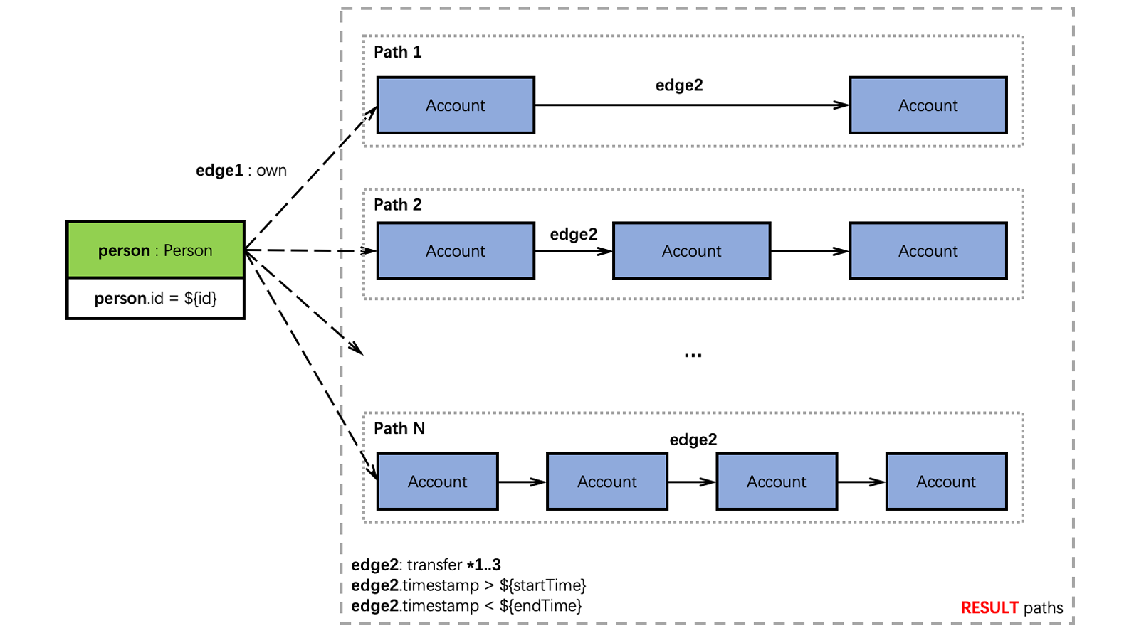
As an illustration of temporal paths, the figure above shows the ExactAccountTransferTrace query of LDBC FINBench: Given a person and a specific time window defined by startTime and endTime, the query finds all transfer traces originating from an account (src) owned by that person to another account (dst) within at most three steps. Each transfer along the trace must follow strictly increasing timestamps, ensuring temporal order. 

Such algorithms are essential for influence propagation, temporal causality analysis, and understanding information diffusion across dynamic networks.

Dynamic Graph Embedding and Predictive Learning
Embedding nodes in a vector space enables ML on evolving graphs. Given a sequence of snapshots \(\{G_1, G_2, ..., G_T\}\), embeddings \(\mathbf{z}_v^t\) for node \(v\) at time \(t\) can be learned via temporal extensions of graph neural networks:
\[
\mathbf{z}_v^t = \mathrm{GNN}(\mathbf{z}_{v}^{t-1}, \mathbf{h}_{\mathcal{N}(v)}^t)
\]
where \(\mathbf{h}_{\mathcal{N}(v)}^t\) aggregates neighbor features at time \(t\). Methods like EvolveGCN update GNN parameters over time, allowing embeddings to capture both structure and temporal dynamics. These embeddings support link prediction, anomaly detection, and node-level forecasting in a dynamic setting. For example, predicting whether a future edge \((u, v)\) will appear can be formulated as:
\[
\hat{y}_{uv}^{t+1} = \sigma(\mathbf{z}_u^t \cdot \mathbf{z}_v^t)
\]
where \(\sigma\) is the sigmoid function. By leveraging temporal embeddings, predictive tasks gain a dynamic, history-aware perspective unavailable in static representations.

Algorithmic Challenges

Working with dynamic graphs is more challenging than static graphs because you must handle:

• Efficiently updating metrics rather than full recompute.
• Incorporating both temporal and structural dependencies.
• The scale: high‐frequency updates and large graphs.
• Deciding temporal granularity: too coarse may miss events; too fine may overwhelm computation.

In practice, a combined strategy is used: data structures that support streaming or incremental updates + algorithms tailored for temporal patterns + modeling frameworks that preserve time, structure and features.

Visualization of Dynamic Graphs

Visualizing dynamic graphs is crucial for understanding how network structures unfold over time, revealing temporal patterns and anomalies that static views cannot capture.

Animation for Temporal Dynamics

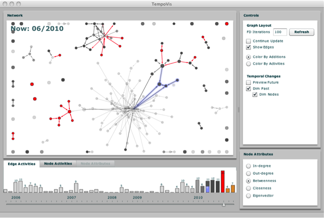
In this example (from Cambridge Intelligence’s KeyLines / ReGraph), nodes represent entities such as people, accounts, or devices, and edges represent time-stamped interactions between them, like transactions or communications. The animation uses a stable layout with a time slider so nodes and edges can appear or fade as they become active or inactive.

Animation helps visualize how nodes and edges evolve, appear, or disappear over time. By presenting sequential frames, it reveals patterns such as emerging communities, shifting influence, or short-lived interactions. A stable layout is essential; smooth transitions preserve the viewer’s mental map and make temporal changes intuitive rather than confusing.

Animations work best for small or medium networks where motion remains interpretable. They allow users to observe peaks of activity, structural shifts, or changes in centrality. But as networks grow, movement becomes overwhelming, and animation alone may fail to convey structure clearly, requiring more static or aggregated views.

Timeline and Snapshot Views

Here, nodes are entities and edges are time-bound interactions shown across different time slices. The snapshot layout, inspired by Cambridge Intelligence’s hybrid approach, uses small multiples plus a timeline control to let analysts compare structural changes over time without relying on animation.

Timeline and snapshot visualizations display a network at multiple time steps without animation. Arranged side by side or stacked, these views highlight how clusters emerge, dissolve, or reorganize. They help analysts compare structural changes across time, providing clarity even when networks are large or densely connected.

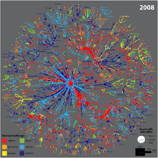
This example (from a trajectory visualization system) maps trajectories to horizontal bands, where color encodes an attribute of each trajectory (e.g., curvature). Similarly, in edge–time heatmaps, edges between nodes can be tracked over time, with color reflecting interaction strength or presence.

Edge–time heatmaps offer another perspective, mapping nodes or node pairs against time. Colors encode interaction strength or presence, making bursts of activity or quiet periods easy to detect. These temporal-focused views avoid spatial clutter and are especially valuable for dense networks where traditional layouts obscure meaningful patterns.

Tracing Evolution and Multilayer Views

In this multilayer view, nodes are entities and intralayer edges represent time-stamped interactions within a layer, while temporal links connect the same node across layers. Each layer shows the network at a distinct time step, enabling analysts to track how neighborhoods and communities evolve over time.

Evolution traces follow selected nodes or edges, showing how neighborhoods grow, shrink, or shift. They highlight changes in connectivity, attributes, or influence over time. This targeted view reveals local dynamics that broader visualizations may miss, helping analysts understand behavior at the level of specific entities.

Multilayer visualizations represent each time step as a distinct layer connected by temporal links. This structure captures how communities merge, split, or transition. Combined with filtering or aggregation, multilayer views maintain clarity in complex datasets. Tools such as Gephi and temporal network libraries support these techniques effectively.

Applications of Dynamic Graphs

Dynamic graphs are practically indispensable in many modern domains. Below are selected application areas illustrating how modeling temporal change adds value.

Cybersecurity and Fraud Detection
Dynamic graphs are vital in cybersecurity and fraud detection because user, device, and transaction relationships change constantly. By processing events in real time, they capture anomalies such as sudden spikes in connections or tightly formed clusters that indicate coordinated attacks. Incorporating temporal information also enables prediction of attack paths and reduces false positives, helping organizations understand how threats evolve and respond more effectively.

Social Networks and Communication Systems
Social and communication networks are inherently dynamic, with users, interactions, and content flows changing continuously. Modeling them as dynamic graphs reveals patterns like viral cascades, transient communities, and evolving influence that static views miss. Temporal analysis supports link prediction, community detection, traffic optimization, and anomaly detection, offering deeper insight into user behavior and overall network health.

Artificial Intelligence and Machine Learning
Dynamic graphs are key in AI systems that rely on evolving relational data, such as social networks, knowledge graphs, and recommendation engines. Techniques like temporal embeddings and dynamic graph neural networks integrate historical context and update representations as the graph evolves. This improves link prediction, anomaly detection, and influence modeling, enabling AI systems to anticipate future interactions, detect emerging trends, and adapt more effectively to real-world temporal changes.

Challenges in Dynamic Graph Analysis

Analyzing dynamic graphs offers powerful insights but introduces several unique challenges that researchers and practitioners must navigate to ensure accurate, scalable, and interpretable results.

Temporal Granularity and Storage
Choosing the right temporal resolution is critical. Coarse snapshots may overlook short-lived events, while fine-grained event logs increase storage demands. Maintaining long sequences of graph snapshots or high-frequency event streams can quickly consume disk space and memory, making efficient representation and compression strategies essential for practical analysis.

Algorithmic Complexity
Dynamic graphs require algorithms that adapt to continuous changes. Unlike static computations, metrics like centrality, reachability, or clustering must update incrementally. Designing incremental or streaming algorithms that balance accuracy with speed is challenging, especially as graphs grow in size and update frequency, demanding careful trade-offs between computation and responsiveness.

Concept Drift and Non-Stationarity
Graph properties evolve over time: node roles, edge distributions, and community structures can shift. Models trained on historical snapshots may become outdated, reducing predictive accuracy. Handling such non-stationarity requires continuous monitoring, adaptive models, and mechanisms to detect and respond to concept drift without overfitting to transient fluctuations.

Visualization and Interpretability
Representing temporal evolution clearly is difficult. Animated layouts can preserve context but may overwhelm viewers in large networks. Alternative methods, like timeline views, multilayer graphs, or heatmaps, help highlight trends and temporal patterns. Balancing visual clarity with completeness is crucial to make evolving network structures understandable and actionable.

PuppyGraph: Create Dynamic Graphs Directly on Your Existing Data

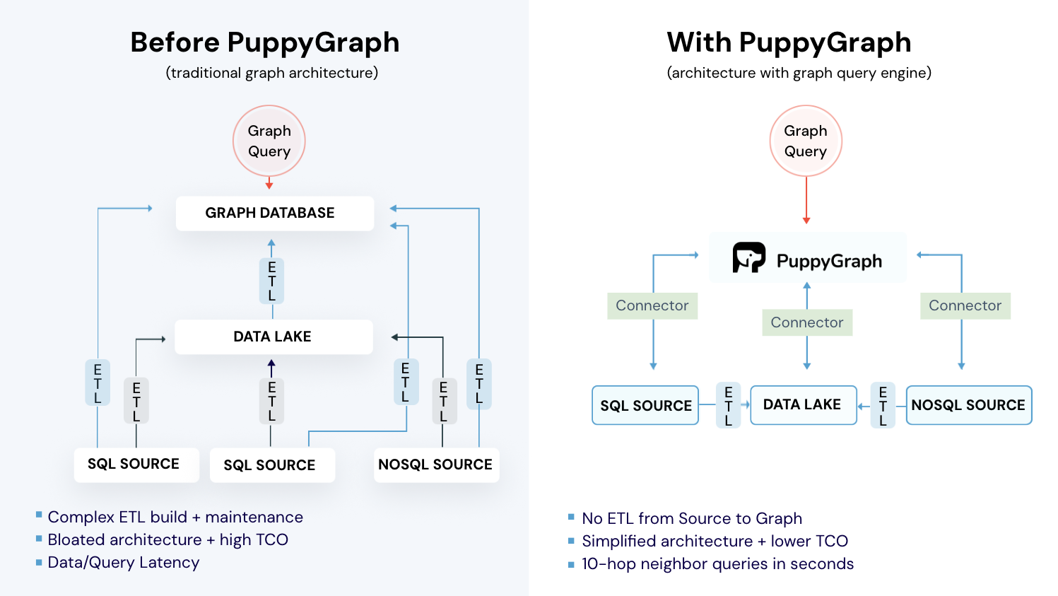
In fast-moving domains, especially cybersecurity and finance, data grows rapidly and relationships between entities change constantly, forming dynamic graphs. Traditional solutions require data to be loaded into a graph engine via complex ETL pipelines, delaying insights. PuppyGraph eliminates this step by integrating streaming sources such as StreamNative, RisingWave, and Redpanda, enabling real-time graph queries with Gremlin or openCypher, delivering instant, interactive insights on continuously evolving data, no ETL, no delays.

PuppyGraph is the first and only real time, zero-ETL graph query engine in the market, empowering data teams to query existing relational data stores as a unified graph model that can be deployed in under 10 minutes, bypassing traditional graph databases' cost, latency, and maintenance hurdles.

It seamlessly integrates with data lakes like Apache Iceberg, Apache Hudi, and Delta Lake, as well as databases including MySQL, PostgreSQL, and DuckDB, so you can query across multiple sources simultaneously.

Key PuppyGraph capabilities include:

• Zero ETL: PuppyGraph runs as a query engine on your existing relational databases and lakes. Skip pipeline builds, reduce fragility, and start querying as a graph in minutes.

• No Data Duplication: Query your data in place, eliminating the need to copy large datasets into a separate graph database. This ensures data consistency and leverages existing data access controls.

• Real Time Analysis: By querying live source data, analyses reflect the current state of the environment, mitigating the problem of relying on static, potentially outdated graph snapshots. PuppyGraph users report 6-hop queries across billions of edges in less than 3 seconds.

• Scalable Performance: PuppyGraph’s distributed compute engine scales with your cluster size. Run petabyte-scale workloads and deep traversals like 10-hop neighbors, and get answers back in seconds. This exceptional query performance is achieved through the use of parallel processing and vectorized evaluation technology. 

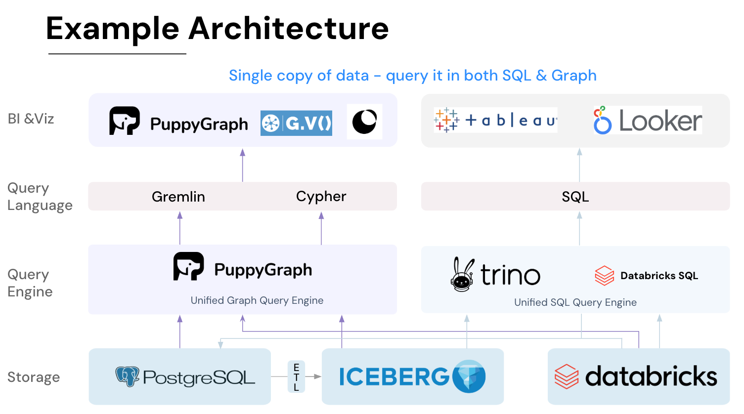
• Best of SQL and Graph: Because PuppyGraph queries your data in place, teams can use their existing SQL engines for tabular workloads and PuppyGraph for relationship-heavy analysis, all on the same source tables. No need to force every use case through a graph database or retrain teams on a new query language.
• Lower Total Cost of Ownership: Graph databases make you pay twice — once for pipelines, duplicated storage, and parallel governance, and again for the high-memory hardware needed to make them fast. PuppyGraph removes both costs by querying your lake directly with zero ETL and no second system to maintain. No massive RAM bills, no duplicated ACLs, and no extra infrastructure to secure.

• Flexible and Iterative Modeling: Using metadata driven schemas allows creating multiple graph views from the same underlying data. Models can be iterated upon quickly without rebuilding data pipelines, supporting agile analysis workflows.

• Standard Querying and Visualization: Support for standard graph query languages (openCypher, Gremlin) and integrated visualization tools helps analysts explore relationships intuitively and effectively.

• Proven at Enterprise Scale: PuppyGraph is already used by half of the top 20 cybersecurity companies, as well as engineering-driven enterprises like AMD and Coinbase. Whether it’s multi-hop security reasoning, asset intelligence, or deep relationship queries across massive datasets, these teams trust PuppyGraph to replace slow ETL pipelines and complex graph stacks with a simpler, faster architecture.

As data grows more complex, the most valuable insights often lie in how entities relate. PuppyGraph brings those insights to the surface, whether you’re modeling organizational networks, social introductions, fraud and cybersecurity graphs, or GraphRAG pipelines that trace knowledge provenance.

Deployment is simple: download the free Docker image, connect PuppyGraph to your existing data stores, define graph schemas, and start querying. PuppyGraph can be deployed via Docker, AWS AMI, GCP Marketplace, or within a VPC or data center for full data control.

Conclusion

Dynamic graphs fundamentally change how we understand complex systems. By modeling how nodes, edges, and attributes evolve over time, they reveal temporal patterns, causal chains, and structural changes that static snapshots simply cannot capture. From social interactions and financial transactions to communication flows and biological processes, incorporating time unlocks a deeper, more realistic view of how real-world networks behave.

To harness these insights in real time, PuppyGraph makes dynamic graph analysis practical and scalable. By querying existing data directly without ETL, PuppyGraph supports incremental updates, temporal reasoning, and large-scale graph exploration, turning evolving data into operational advantages. Explore the forever free PuppyGraph Developer Edition or book a demo to see how it can transform your dynamic data into actionable insights.