Join Out of Memory: How To Fix?

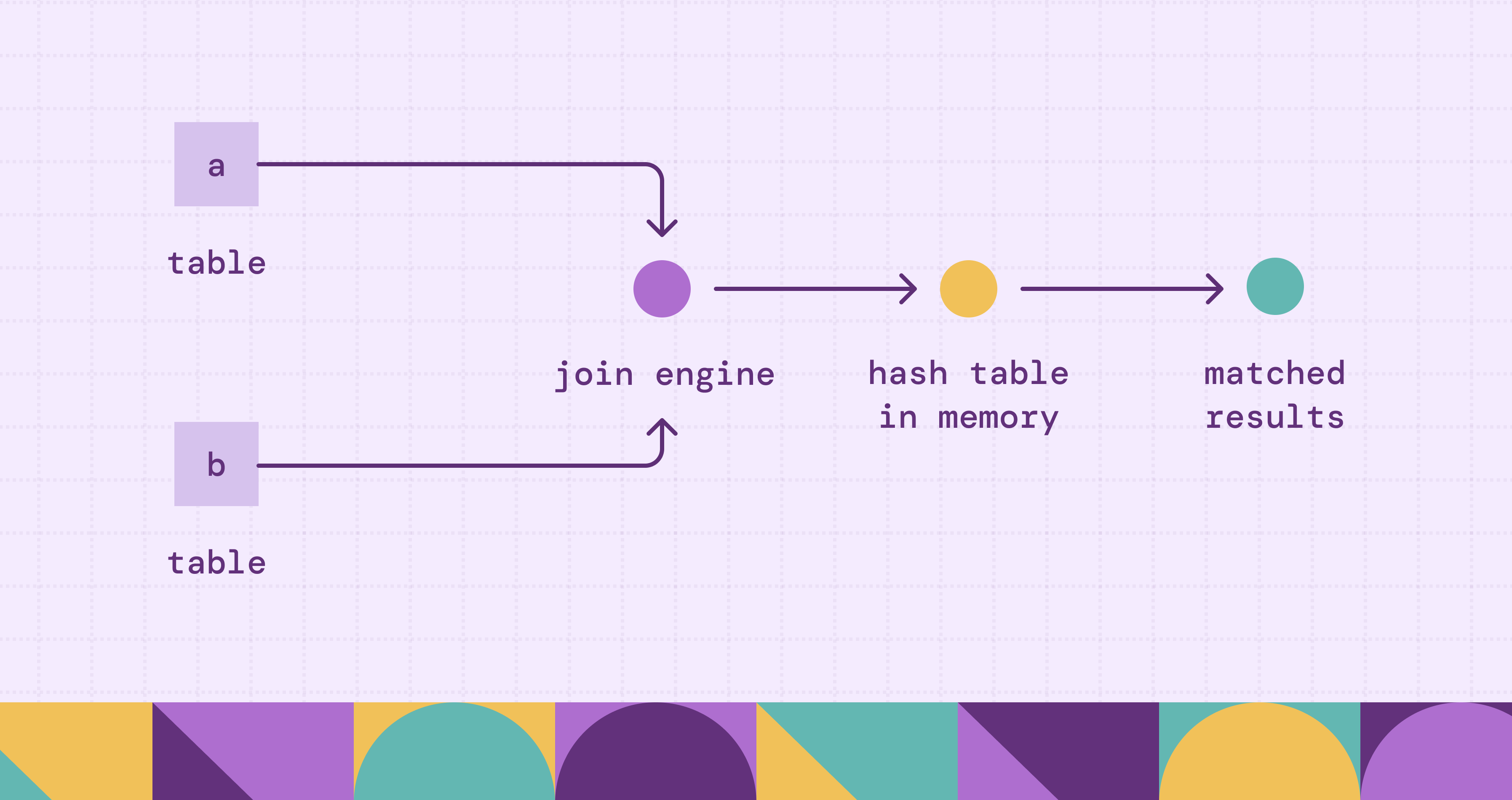
Data platforms frequently encounter “join out of memory” errors when SQL joins require more memory than execution engines can allocate. As datasets grow larger and more complex, join operations become increasingly expensive due to hash tables, shuffle stages, intermediate buffers, and skewed key distributions. Poor query design, oversized datasets, and inefficient execution strategies can quickly overwhelm distributed systems such as Spark, Hive, PostgreSQL, and BigQuery.

This article explains why SQL joins consume significant memory and how different join strategies contribute to memory failures. It further explores key factors including hash joins, shuffle joins, data skew, partitioning, bucketing, indexing, and query optimization techniques. By understanding these mechanisms and applying practical optimization methods, engineers can significantly reduce memory pressure and improve join performance in large-scale analytical environments.

What Does “Join Out of Memory” Mean?

A “Join Out of Memory” error occurs when a database or distributed processing engine cannot allocate enough memory to complete a join operation. During execution, the engine typically loads part of one or both datasets into memory to match rows efficiently. If the required memory exceeds available limits, the query fails.

Different systems display different error messages. Apache Spark may show ExecutorLostFailure or Java heap space exceptions. Hive can throw GC overhead limit exceeded. PostgreSQL may report insufficient work_mem, while BigQuery may fail with shuffle resource exhaustion. Although the wording varies, the root cause remains the same: the join operation requires more memory than the system can provide.

The issue usually appears when queries process massive tables, poorly filtered datasets, or highly skewed keys. Even moderately sized joins can fail if execution plans are inefficient. For example, selecting unnecessary columns or joining before filtering data can dramatically increase memory pressure. In distributed systems, memory usage also includes shuffle buffers, hash tables, serialization overhead, and intermediate result storage.

The following diagram illustrates how a join operation consumes memory during execution:

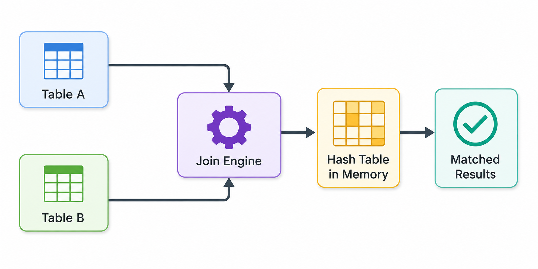
A join becomes problematic when the hash table or shuffle stage grows larger than available executor memory. This is especially dangerous in cloud-native data platforms where parallel workers exchange huge volumes of intermediate data across the network.

Why SQL Joins Consume Large Amounts of Memory

Joins are fundamentally expensive because they require comparing rows across datasets. Unlike simple filtering or aggregation operations, joins often require engines to temporarily reorganize, copy, sort, or hash large amounts of data before matching records can be produced.

The amount of memory consumed depends on several variables. Dataset size is the most obvious factor, but row width is equally important. A table with 100 million rows and 50 columns can consume dramatically more memory than a table with the same row count and only 5 columns. Wide string columns, JSON payloads, and nested structures amplify memory usage further.

Another major factor is the join type. Inner joins, left joins, cross joins, and many-to-many joins all behave differently. Cross joins are particularly dangerous because they generate Cartesian products. If two datasets each contain one million rows, a cross join could theoretically create one trillion output rows.

Execution engines also need temporary structures during processing. Hash joins build in-memory hash maps. Sort-merge joins allocate buffers for sorting operations. Distributed joins create shuffle files and network buffers. Even if the final output is relatively small, intermediate processing stages can require enormous memory allocations.

Consider this simplified SQL example:

SELECT *
FROM orders o
JOIN customers c
ON o.customer_id = c.customer_id;

At first glance, the query seems harmless. However, if both tables contain billions of rows and lack filtering predicates, the engine may need to redistribute and hash massive datasets across worker nodes. The join itself becomes a memory-intensive operation even before results are returned.

Poor query design magnifies the problem. Joining tables before filtering, selecting unnecessary columns, or failing to use partition pruning can multiply memory requirements several times over.

Understanding Hash Joins and Memory Usage

Hash joins are among the most common join algorithms in modern analytical systems because they are efficient for large unsorted datasets. However, they are also one of the leading causes of out-of-memory failures.

In a hash join, the engine first selects a smaller table as the build side. It loads this table into memory and creates a hash table using the join key. The larger table becomes the probe side. Each row from the probe side is scanned and matched against the in-memory hash structure.

The process looks like this:

Hash joins are extremely fast when the build-side table fits comfortably into memory. Problems arise when the supposedly “small” table is still very large. If the hash table exceeds executor memory, the system either spills to disk or crashes entirely.

Spark attempts to spill oversized hash structures to disk, but performance degrades sharply when this happens. Hive and Presto behave similarly. PostgreSQL uses work_mem thresholds before switching strategies. BigQuery dynamically allocates slots but can still encounter shuffle resource exhaustion during oversized joins.

Memory usage also increases when join keys contain high-cardinality strings or complex nested objects. Integer-based joins are far more memory efficient than joins involving large VARCHAR fields or serialized JSON values.

Another overlooked issue is duplicate keys. If one key appears millions of times, the corresponding hash bucket becomes extremely large, creating memory hotspots inside executors.

One practical optimization is reducing the build-side dataset before joining:

SELECT *
FROM large_sales s
JOIN (
    SELECT customer_id, region
    FROM customers
    WHERE active = true
) c
ON s.customer_id = c.customer_id;

By filtering inactive customers first, the hash table becomes much smaller, reducing memory consumption significantly.

How Large Datasets Trigger Memory Failures

Large datasets are the most obvious trigger for join memory failures, but the underlying mechanics are more complex than simply “too much data.” The real issue comes from intermediate processing stages growing beyond system capacity.

Distributed engines divide datasets into partitions processed by worker nodes. During joins, rows sharing the same join key must often be moved to the same node. This redistribution process, called shuffling, creates massive temporary datasets that consume memory, network bandwidth, and disk space simultaneously.

Imagine joining two 5 TB datasets on a non-partitioned column. The engine may need to reshuffle almost all rows across the cluster. Even if each executor handles only a fraction of the data, the cumulative memory pressure becomes enormous.

Large datasets also increase garbage collection overhead in JVM-based systems like Spark and Hive. Executors constantly allocate and free temporary objects during joins. When memory becomes saturated, garbage collection cycles intensify, slowing execution dramatically before eventual failure.

The following workflow illustrates the issue:

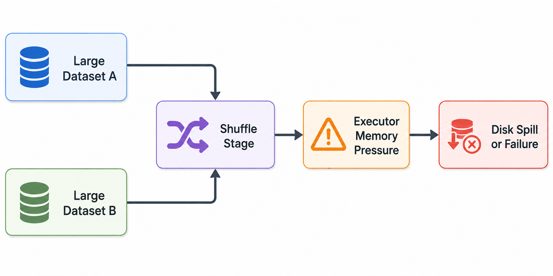
Another problem is insufficient partitioning. If datasets are stored in very few partitions, individual executors receive oversized workloads. Conversely, excessive partition counts can increase scheduling overhead and shuffle metadata size.

Cloud environments introduce additional complexity because memory allocation is often fixed per worker node. Queries that exceed configured limits cannot automatically scale upward unless autoscaling policies are enabled.

Data engineers sometimes assume adding more cluster nodes solves the problem. In reality, poor join design can still overload executors regardless of cluster size. Efficient query planning matters more than raw hardware in many scenarios.

Broadcast Join vs Shuffle Join Memory Issues

Broadcast joins and shuffle joins represent two fundamentally different execution strategies. Understanding their tradeoffs is critical for avoiding memory failures.

In a broadcast join, the smaller dataset is copied to every worker node. Each executor stores the entire smaller table locally and joins it with partitions of the larger dataset. This approach avoids expensive shuffling and is extremely fast when the broadcast table is truly small.

Spark automatically uses broadcast joins for small tables under a configurable threshold. BigQuery and Snowflake implement similar optimizations internally.

Example:

SELECT /*+ BROADCAST(customers) */
*
FROM sales
JOIN customers
ON sales.customer_id = customers.customer_id;

Broadcast joins reduce network overhead dramatically, but they can create memory issues if the broadcast table is larger than expected. Since every executor receives a copy, memory consumption multiplies across the cluster.

Shuffle joins behave differently. Instead of broadcasting one table, both datasets are repartitioned based on the join key. Matching rows are moved to the same executor for processing.

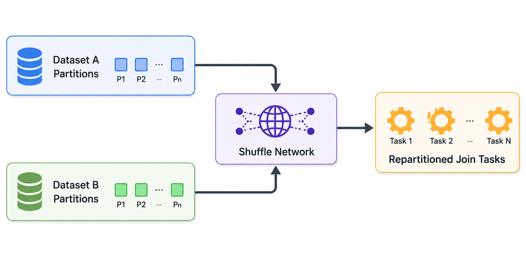
Shuffle joins scale better for very large datasets but require enormous temporary memory and network buffers. If shuffle partitions become uneven or oversized, executors may crash due to memory exhaustion.

Broadcast joins typically fail because of insufficient executor heap memory. Shuffle joins fail because of shuffle spill overload, skewed partitions, or network resource exhaustion.

Choosing the correct strategy depends on table size, partition distribution, and available cluster memory. Many systems allow manual join hints so engineers can override poor optimizer decisions.

How Data Skew Causes Join Memory Problems

Data skew is one of the most underestimated causes of join failures. Skew occurs when certain join keys appear far more frequently than others. Instead of work being evenly distributed across executors, a few partitions become disproportionately large.

For example, imagine an e-commerce dataset where millions of transactions share the same country code or product category. During repartitioning, all rows with the same key may end up on a single executor. That node becomes overloaded while others remain mostly idle.

A skewed join can cause severe memory imbalance even if the total dataset size is manageable. One executor may receive 90% of the workload and run out of memory while the rest of the cluster sits underutilized.

The problem can be visualized like this:

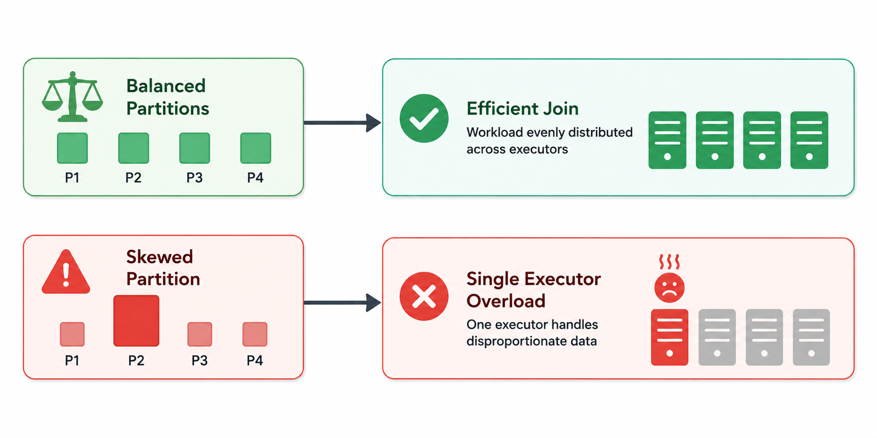
Spark includes adaptive query execution (AQE) features to mitigate skew by splitting oversized partitions dynamically. Hive and Presto offer skew join optimizations as well. However, these features are not always enabled by default.

A common mitigation strategy is salting. Salting artificially distributes skewed keys across multiple partitions by appending random suffixes.

Example:

SELECT *
FROM orders o
JOIN customers c
ON CONCAT(o.customer_id, RAND()) =
   CONCAT(c.customer_id, RAND());

Although salting increases complexity, it spreads skewed records more evenly across executors.

Filtering skewed keys separately can also help. In some cases, processing extremely common keys independently prevents catastrophic executor overload during the main join operation.

Understanding key distribution before joining is therefore essential. Even well-indexed queries can fail if skew is ignored.

Techniques to Reduce Join Memory Consumption

Reducing join memory usage starts with minimizing the amount of data participating in the join. The fewer rows and columns processed, the smaller the intermediate structures become.

Projection pruning is one of the simplest yet most effective optimizations. Instead of selecting entire rows, queries should include only necessary columns.

Bad practice:

SELECT *
FROM sales
JOIN customers
ON sales.customer_id = customers.customer_id;

Better approach:

SELECT *
FROM sales
JOIN customers
ON sales.customer_id = customers.customer_id;

Filtering data before joins is equally important. Predicate pushdown reduces input size dramatically, lowering both shuffle volume and hash table size.

Compression and efficient file formats also matter. Columnar storage formats such as Parquet and ORC reduce memory footprint because engines load only relevant columns into memory.

Caching should be used carefully. While caching can improve performance for reused datasets, caching oversized tables may worsen memory pressure and increase garbage collection overhead.

Another effective strategy is breaking large joins into smaller stages. Instead of one monolithic query joining many huge tables simultaneously, engineers can materialize intermediate filtered datasets.

Approximate algorithms can sometimes replace joins entirely. Bloom filters, semi-joins, and probabilistic matching techniques reduce data movement significantly in distributed systems.

Memory tuning parameters also help. Spark configurations such as:

spark.sql.shuffle.partitions
spark.executor.memory
spark.memory.fraction

can improve join stability when properly adjusted.

However, increasing memory alone is rarely sufficient. Query design and data layout usually produce greater improvements than simply allocating larger executors.

Partitioning and Bucketing for Efficient Joins

Partitioning and bucketing are among the most powerful techniques for improving join efficiency in large-scale systems. Proper data organization reduces shuffle operations, lowers memory consumption, and accelerates query execution.

Partitioning divides tables into physical segments based on column values. Queries filtering on partition keys can skip irrelevant partitions entirely, reducing the amount of data scanned during joins.

For example:

CREATE TABLE sales (
    order_id BIGINT,
    customer_id BIGINT,
    order_date DATE
)
PARTITIONED BY (order_date);

If a query only analyzes recent dates, older partitions are ignored automatically.

Bucketing works differently. Instead of storing rows by value ranges, bucketing hashes rows into fixed groups based on join keys.

CLUSTERED BY (customer_id)
INTO 32 BUCKETS;

When two tables share the same bucketing strategy, engines can perform bucket-aware joins without reshuffling data extensively. This optimization significantly reduces network overhead and executor memory pressure.

The following diagram shows the difference:

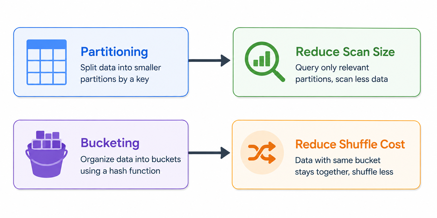
Partitioning is especially effective for time-series datasets. Bucketing is particularly valuable for frequently joined dimension tables.

However, over-partitioning creates problems of its own. Thousands of tiny partitions increase metadata overhead and reduce execution efficiency. Engineers must balance partition granularity carefully.

Modern lakehouse systems such as Delta Lake, Iceberg, and Hudi extend these concepts further with adaptive clustering and data skipping indexes, enabling even more efficient large-scale joins.

Query Optimization Strategies for Large Joins

Efficient query design often matters more than hardware scaling. Many out-of-memory issues can be solved through better optimization strategies without increasing cluster size.

Join order is one of the most critical factors. Optimizers usually attempt to join smaller filtered datasets first, but manual restructuring sometimes produces better results.

For example:

WITH filtered_sales AS (
    SELECT *
    FROM sales
    WHERE order_date >= '2025-01-01'
)
SELECT *
FROM filtered_sales s
JOIN customers c
ON s.customer_id = c.customer_id;

Filtering first drastically reduces join input size.

Semi-joins and EXISTS clauses are often more memory efficient than full joins when only existence checks are needed.

Example:

SELECT customer_id
FROM customers c
WHERE EXISTS (
    SELECT 1
    FROM sales s
    WHERE s.customer_id = c.customer_id
);

This avoids materializing large joined datasets unnecessarily.

Adaptive query execution is another powerful optimization available in Spark 3.x and newer systems. AQE dynamically changes execution strategies based on runtime statistics. It can convert shuffle joins into broadcast joins automatically or split skewed partitions during execution.

Statistics collection is equally important. Optimizers rely on accurate table statistics to choose efficient join plans. Outdated statistics often lead to catastrophic execution decisions.

In distributed environments, reducing shuffle partitions improves performance for smaller joins, while increasing partitions may help balance extremely large workloads. Fine-tuning partition counts based on cluster size is essential for stable execution.

Materialized views and pre-aggregated tables can also eliminate expensive joins entirely in analytical workloads.

Indexing Techniques to Improve Join Performance

Indexes improve join performance by reducing the amount of data scanned during lookup operations. While indexing is more common in traditional relational databases than distributed data lakes, it remains highly relevant for memory optimization.

B-tree indexes are the standard choice for equality joins and range queries. When join keys are indexed, the database can locate matching rows quickly without scanning entire tables.

Example:

CREATE INDEX idx_customer_id
ON customers(customer_id);

Bitmap indexes are especially useful in analytical systems containing low-cardinality columns such as gender, region, or status flags. They reduce memory usage by representing values compactly.

Distributed systems use alternative indexing mechanisms. Delta Lake employs data skipping statistics. Apache Iceberg tracks partition metadata aggressively. BigQuery uses clustering to organize related rows physically.

Covering indexes are particularly powerful because they include all columns required by a query, eliminating additional table lookups.

However, indexes also introduce tradeoffs. Maintaining indexes increases storage overhead and slows insert operations. Excessive indexing can hurt ETL performance in write-heavy environments.

Indexes alone cannot solve large join problems if datasets still require extensive shuffling. They work best when combined with partitioning, filtering, and efficient execution strategies.

The relationship between indexing and joins can be summarized as follows:

Analytical databases increasingly combine indexing with vectorized execution and columnar compression to improve join efficiency further.

When SQL Joins Become Difficult to Manage

Modern SQL engines have become highly efficient at executing joins at scale. Systems such as Spark, Snowflake, BigQuery, and Hive can optimize shuffle strategies, rebalance skewed partitions, and dynamically choose between broadcast joins and hash joins to improve performance and reduce memory pressure.

However, efficient execution does not eliminate every join-related challenge.

As enterprise SQL environments grow, joins increasingly become the mechanism through which relationships are represented across datasets. Over time, these relationships become scattered across ETL pipelines, dashboards, application logic, and analyst-written SQL, making join logic increasingly difficult to manage consistently.

The underlying challenge is that SQL joins primarily describe how records can be connected through matching keys, but they do not always clearly describe the semantics of those relationships.

This is where a semantic layer becomes useful. 

The Role of a Semantic Layer

A semantic layer sits above existing SQL systems and exposes business concepts directly, such as Customer, Order, Product, Supplier, or Transaction. Instead of forcing applications or AI systems to reason through raw tables and complex joins, the semantic layer provides a higher-level logical model aligned with business meaning.

This allows developers, analysts, and AI agents to work with data more naturally without changing the underlying SQL infrastructure.

Ontology and Ontology Enforcement

At the core of many semantic layers is an ontology: a formal definition of entities, relationships, and rules across the SQL data environment. An ontology defines what entities exist, how they relate to one another, and what relationships are valid.

For example, a Customer may place an Order, an Order may contain a Product, and a Supplier may provide that product. While SQL joins can technically connect many tables together, ontology enforcement ensures that queries and updates follow semantically valid relationships rather than relying only on matching keys.

Whether data operations originate from applications, analysts, or AI systems, ontology-aware systems can validate interactions against the semantic model to reduce inconsistent or logically invalid results.

Why It Matters: From Join Complexity to Semantic Clarity

Without a semantic layer, the complexity of SQL joins often shifts into application logic and orchestration layers, making systems harder to maintain as datasets and relationships grow.

For AI systems, the challenge becomes even greater. Large language models and autonomous agents may generate syntactically correct SQL queries while still misunderstanding the actual meaning of relationships between tables. An AI system can successfully execute a join operation yet produce results that are logically incorrect from a business perspective.

This creates what might be described as semantic fog: navigating ambiguous schemas, undocumented joins, inconsistent naming conventions, and unclear entity relationships across large SQL environments.

Ontology enforcement acts as a semantic guardrail, helping ensure that AI-generated reads and writes follow validated business relationships instead of relying solely on physical table connections. Rather than returning only low-level database errors, ontology-aware systems can provide structured semantic feedback that helps AI systems refine and correct their behavior over time.

Data Access with AI Assistants

Moving beyond query optimization alone, platforms such as PuppyGraph provide a graph-based way to access and query existing SQL data as connected knowledge without requiring organizations to migrate data into a separate graph database.

This enables developers and AI systems to explore relational data through graph-style reasoning and relationship-aware retrieval while continuing to use existing SQL and lakehouse infrastructure.

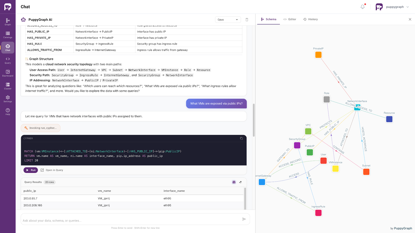
Powered by the same ontology-enforced foundation, this approach supports more context-aware access to enterprise data. It allows AI systems to interpret user intent within a well-defined semantic framework and retrieve information accordingly.

As a result, enterprise SQL data evolves from a passive storage layer into an active semantic layer: one that preserves consistency while enabling more reliable analytics, search, and next-generation AI applications.

Conclusion

SQL join out-of-memory errors are not caused by a single issue but by the combined impact of large datasets, inefficient execution strategies, data skew, excessive shuffling, and poor query design. Understanding how hash joins, broadcast joins, partitioning, bucketing, indexing, and adaptive optimization affect memory consumption is essential for building stable and scalable analytical systems. In most cases, reducing data volume before joins and optimizing data layout are more effective than simply adding more hardware resources.

As SQL environments continue to grow in complexity, the challenge extends beyond execution performance to managing the meaning of relationships across datasets. Semantic layers and ontology enforcement help organizations move from low-level join logic toward business-aware data access. By combining optimized SQL infrastructure with semantic understanding, platforms such as PuppyGraph enable more reliable analytics, clearer data relationships, and more context-aware AI applications.

Explore the forever-free PuppyGraph Developer Edition, or book a demo to see how PuppyGraph transforms complex SQL joins into semantic, graph-powered data access. 

‍