Neo4j Scalability: Architecture, Performance

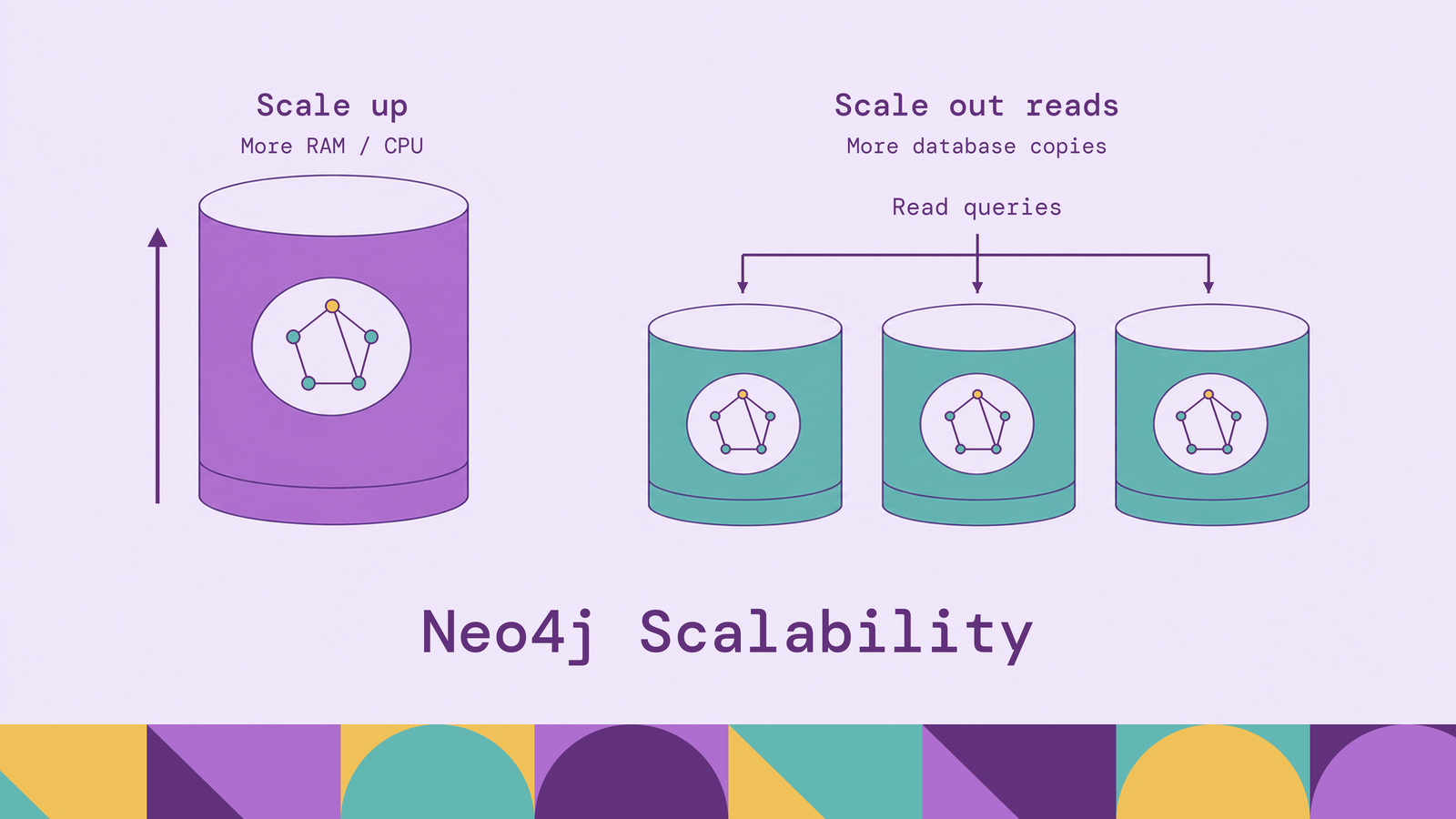
Neo4j scales asymmetrically. Reads scale out across replicated copies of a database, writes are bounded by a single elected leader, and one graph is bounded by what a single server can hold, until you cut it into pieces that can no longer traverse each other freely. That follows from the design choice that makes the engine fast: relationships are stored next to the nodes they connect, so a hop is a pointer dereference rather than a join, and locality is what a partition boundary destroys.

This post covers what scalability means for a graph workload, the architecture beneath Neo4j’s scaling options, how clustering and sharding distribute load, and what governs query performance.

What is Neo4j scalability?

Scalability for a graph database is four properties, and a deployment can be comfortable on three while failing on the fourth: data volume, how much graph the system holds and still serves; read concurrency, how many simultaneous queries it answers; write throughput, how many transactions per second it commits; and query complexity, how deep and branchy a traversal can get before latency becomes unacceptable.

The last axis separates graph scalability from relational scalability. Doubling a table’s row count roughly doubles the cost of a scan, while doubling a graph’s node count may not change the cost of a three-hop traversal at all, because the traversal only touches the neighborhood it walks. What degrades instead is a hop that leaves the cached working set, a node whose degree has grown into the millions, or an expansion that fans out faster than its filters cut it down. Plan capacity for those, not for total size.

How does Neo4j scale?

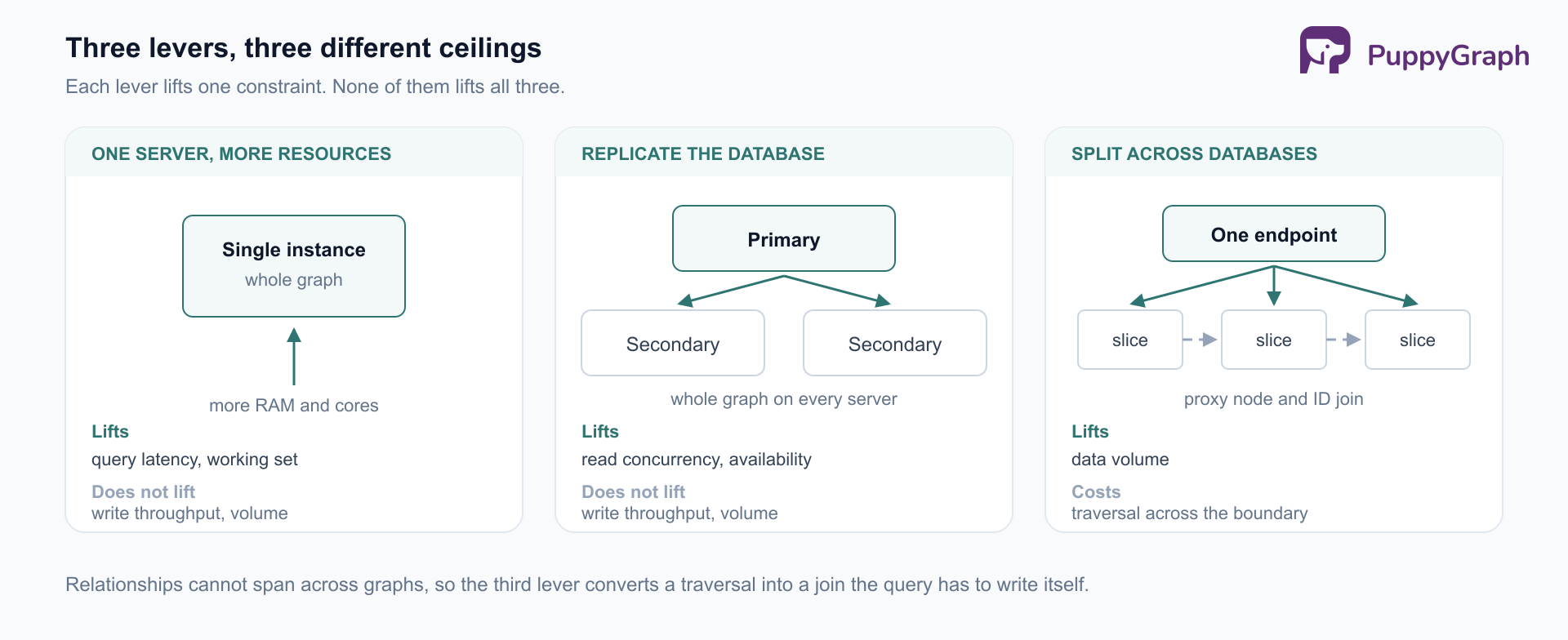
Scaling a Neo4j deployment means working three levers, and they are not interchangeable.

Give one server more resources. A single instance holding its working set in memory is the baseline, and for most graphs the fastest configuration, because no hop crosses a network.

Replicate the database across servers. Additional copies serve reads and provide failover. Neo4j’s scaling guidance lists data volume for a clustered database as limited to single server size, since every copy holds the whole graph.

Split the data across databases. Composite databases federate several databases behind one endpoint; sharded property databases distribute property data across shards. Both lift the volume ceiling, and both put conditions on how queries may be written.

Neo4j scaling architecture

Three architectural facts govern everything above.

Storage is native and adjacency is direct. A relationship is a stored object holding pointers to the nodes at each end, so a hop is a fixed dereference rather than a lookup that grows with the graph. That is what makes deep traversal viable, and why splitting a graph across machines is costly: a pointer that becomes a network call is no longer fixed-cost.

Memory is the real capacity unit. The page cache holds graph and index pages; the heap holds the objects a running query instantiates. Neo4j’s memory configuration guidance is to size the page cache against the data and indexes with room for growth, and to set both explicitly at startup.

Store format sets the hard ceilings. The aligned record format, the Community Edition default, caps how many nodes and relationships a database can hold. The block format, GA in Neo4j 5.16 and the Enterprise default since 5.22, raises that node ceiling by orders of magnitude, removes the relationship ceiling entirely, and improves data locality.

Vertical vs horizontal scaling in Neo4j

Vertical scaling is the primary lever for a single graph, unusually so for a modern database, and RAM is the variable that matters, because it decides whether traversals stay in the page cache. Moving a working set from partially cached to fully cached usually beats any query rewrite.

Horizontal scaling multiplies read capacity, not write capacity, and no database grows beyond one server’s size, since each copy holds the entire graph. Scaling out along the other axes requires partitioning the data.

Neo4j clustering and high availability

Neo4j 5 replaced the Causal Cluster vocabulary, and the change is more than cosmetic. In the current model, primary and secondary are roles held by a copy of a database, not by a server, and a server can be constrained to hold only primaries or only secondaries.

Primary copies form the Raft consensus group for their database. One is elected leader and commits writes, and the rest replicate and stand ready to take over, so losing the leader triggers an election and the database keeps serving while a quorum survives. This is also why adding primaries does not add write throughput: each write must reach a quorum, so a larger primary set buys fault tolerance at the cost of commit latency. Our post on Neo4j’s distributed architecture covers consensus and consistency in more depth.

Clustering is an Enterprise Edition feature; Community Edition runs a single instance hosting one standard database.

Neo4j read replicas and scaling read workloads

Read replica is Neo4j 4.x vocabulary. The current equivalent is a secondary copy of a database, asynchronously replicated from a primary through transaction log shipping. Secondaries take no part in consensus, so they can be added without slowing writes.

Asynchronous replication means secondaries lag. Where a user writes and immediately reads back, Neo4j drivers carry bookmarks, and the server holds the read until the copy serving it has caught up.

A driver fetches a routing table naming the writer and the readers for a database, sending writes to the leader and spreading reads across the rest, and routing policies bias that choice toward a local data center or toward machines reserved for heavy analytical reads. This scales a read-dominated workload well and does nothing for a write-dominated one. The limit is structural.

Neo4j sharding and data distribution

Neo4j does not transparently shard a single graph. It offers two mechanisms, cutting in different directions.

Composite databases are the Neo4j 5 successor to Fabric. A composite database is a virtual database whose constituents are ordinary databases, possibly on different servers, addressed in Cypher through the USE clause. Data is split with neo4j-admin database copy, which filters by label and property.

The constraint that shapes everything else is stated plainly in the documentation: relationships cannot span across graphs. Connecting two constituents means federating them with a proxy node pattern, where a node carrying the full record in one graph appears in the other as a stub holding only its ID, and queries join across the boundary on that ID.

CALL () {
  USE shards.customers
  MATCH (c:Customer {region: 'EMEA'}) RETURN c.customerID AS id
}
CALL (id) {
  USE shards.orders
  MATCH (:Customer {customerID: id})-[:PLACED]->(o:Order) RETURN o
}
RETURN o

That is a join between shards, not a traversal, and it is the cost of the model: the query must know the partition, and any pattern crossing the boundary is rewritten around it. Writes are bounded too: the documentation allows only transactions that write to a single constituent, so there is no atomic write across shards.

Sharded property databases, introduced in Neo4j 2025.12, take the opposite cut. Instead of partitioning the graph, they keep nodes and relationships, without their properties, in a single graph shard and distribute the properties across property shards through a hash function, so property-heavy graphs can grow past one server without turning traversals into cross-shard joins. The conditions are steep: property sharding is not part of standard Enterprise Edition and requires an Infinigraph subscription, it is unavailable on Aura, it requires Cypher 25, and Neo4j’s limitations page notes that MERGE queries perform poorly at meaningful scale.

Partitioning a graph is a modeling decision that surfaces in every query written against it, not a configuration change.

Neo4j scalability for large graphs

Three pressures dominate at size.

Working set against page cache. A billion-node graph whose traffic concentrates on a recent slice can behave well on modest hardware, while a smaller graph with uniformly random access thrashes on larger hardware.

Supernodes. A node whose degree grows into the millions turns one expansion step into a scan of an enormous relationship list, and hubs accumulate this way in practice: a shared country, a popular tag, a default account. The mitigations are modeling changes: split the hub into typed subnodes, or move the discriminator into the relationship type so expansion filters before it fans out.

Analytics memory. Graph Data Science algorithms run over an in-memory projection rather than the store, and that projection lives in the heap, so it is a heap budget rather than a page-cache one. Running analytics beside transactional reads puts the two in competition.

Neo4j query performance and scalability

Query cost is largely decided before execution, by the plan. The Cypher planner is cost-based and works from stored statistics and cardinality estimates, choosing which pattern element anchors the traversal and which end it expands from. Two queries returning identical results can differ by orders of magnitude on that choice.

Three factors carry most of the difference. Anchoring is whether the query starts from an indexed lookup or a label scan; an index on the starting property is usually the highest-impact change available. Expansion order is whether the planner begins at the selective end of the pattern, since starting from a filter that returns tens of rows beats starting broad. Bounded depth is whether variable-length patterns carry an upper bound; an unbounded -[:KNOWS*]- can enumerate a combinatorial number of paths on a well-connected graph, and that failure arrives suddenly.

The diagnostic is PROFILE, which reports the plan the engine ran with database hits and rows per operator. Database hits are the honest cost metric, since they count storage accesses, which a warm cache would otherwise hide. At size, query scalability is a planning problem before it is a hardware one. A plan that anchors and bounds its expansion stays cheap as the graph grows; one that does not gets more expensive with every row.

Factors that affect Neo4j scalability

The data model. Label design, relationship types, and property placement decide what the planner can prune and how far an expansion fans out.

Memory and hardware. Page cache and heap sized against the working set, local NVMe, and low latency between cluster members, which enters the commit path for every write.

Concurrency. Writes lock the nodes and relationships they touch, so repeated updates to the same hot nodes serialize regardless of core count.

Edition and deployment. Clustering and composite databases are Enterprise features, property sharding needs an Infinigraph subscription on top, and some options are unavailable on Aura.

Neo4j scalability challenges

Some of these limits are not tuning problems.

The write ceiling is architectural. Past vertical headroom and batching, raising write throughput means splitting data across databases and taking on the constraints of composite databases.

Partitioning fights the data model. Domains with a clean partition key shard well; densely interconnected ones pay for it in proxy nodes and rewritten queries.

Operations scale with the topology. Elections, replication lag, per-database backup, rolling upgrades, and store-format migrations are each manageable, and together a standing cost.

The ingest pipeline scales too. In most enterprise deployments the authoritative data lives in a warehouse, a lakehouse, or operational databases, and the graph is loaded from them by a pipeline. It is a scaling surface of its own, with throughput limits, a staleness window, and its own failure modes.

Neo4j scalability vs other graph databases

The table describes one trade placed three ways. Neo4j’s storage locality is why deep traversal on a single instance is fast and why automatic partitioning is hard. Natively distributed graph databases accept a network hop at partition boundaries as the price of aggregate capacity. Engines over existing storage do not own the layout, so boundary cost reappears as scan and join cost at the source, and they answer no graph writes at all. For a wider survey, see our comparison of the best graph databases.

How to scale Neo4j for enterprise workloads

Measure the working set first. Instrument page cache hit ratio and page faults before buying hardware; a deployment that has fallen out of cache is the most common and most fixable cause of a stalled graph.

Fix the model before the hardware. Profile the slow queries for unanchored patterns and unbounded expansions, and check the degree distribution on hot paths.

Separate workload classes. Route analytical and reporting queries to dedicated secondaries.

Treat partitioning as a design decision, not a switch. Before adopting composite databases, establish that the domain has a partition key most relationships respect; if not, property sharding may fit better.

Scaling analytical reads without replicating the graph

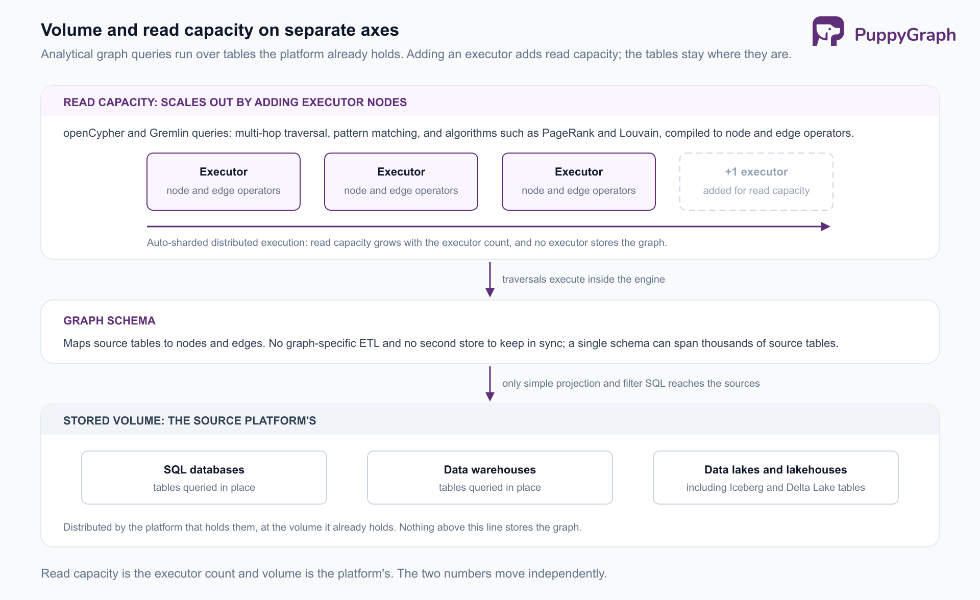
Every lever above scales a copy of the graph: volume is bounded by what one server holds, and read capacity is bought by replicating that whole copy. Where the graph is the system of record for operational writes, that copy is the point, and a native graph database is its right home. Analytical graph work, multi-hop traversal, pattern matching, and algorithms, runs over data the warehouse or lakehouse already holds at volume, and there the copy is the ceiling.

PuppyGraph answers openCypher and Gremlin queries directly against tables that already exist in SQL databases, data warehouses, and data lakes and lakehouses, including open table formats such as Iceberg and Delta Lake. A graph schema maps those tables to nodes and edges, with no graph-specific ETL and no second store to keep in sync, so volume stays the source platform’s: a single graph schema can span thousands of source tables, and deployments run at terabyte to petabyte volume. Read capacity is a separate axis, added by scaling out executor nodes, with auto-sharded distributed execution across them. It sits at the same layer as other SQL query engines in the analytics stack, optimizing for multi-hop traversal and pattern matching rather than relational scans, and standard algorithms such as PageRank and Louvain are callable in queries. A query compiles into a plan of node and edge operators that executes in its own distributed engine, with only simple projection and filter SQL issued to the sources. Because the query is represented as graph operators end to end, the engine optimizes specifically for multi-hop traversals, which is where its traversal performance comes from. Because the engine speaks openCypher over the Bolt protocol, existing Neo4j drivers, applications, and BI tools connect without query rewrites. Volume and read capacity stop being the same number.

Conclusion

Neo4j scales along well-defined axes with clear limits: reads scale out across secondary copies, RAM relative to the working set is the dominant lever for one graph, writes are bounded by a single leader, and growing past one server’s volume means composite databases or property sharding. Most deployments that feel a scaling wall are closer to a working set that no longer fits in the page cache, or an expansion that was never bounded, than to any of those limits.

The question before scaling the cluster is whether the graph needs to be a separate copy of data that already lives elsewhere. Try the forever-free PuppyGraph Developer Edition and book a demo with the team to see how openCypher and Gremlin queries traverse warehouse and lakehouse tables, with no graph-specific ETL, so that read capacity scales by adding executor nodes rather than by replicating the graph.