Snowflake Graph: Architecture, Features & Use Cases

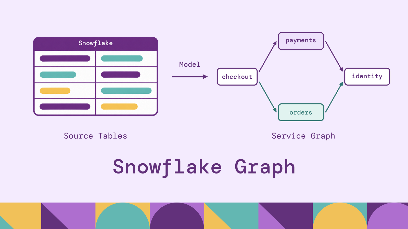
Relationships already stored in Snowflake can answer questions that ordinary summaries leave open: which services depend on a failing component, which accounts share devices, or which suppliers connect otherwise separate product lines. Getting those answers requires a model that preserves connections and queries that follow them across multiple steps.

This guide explains graph modeling over Snowflake warehouse tables, the architecture behind SQL and graph-engine approaches, and how to build and query a small service dependency graph. It also covers where SQL aggregation helps and where more involved graph analytics require a different execution approach.

What is Snowflake graph?

In this article, Snowflake graph means a graph analysis solution built around Snowflake warehouse data. The phrase describes how data is modeled and queried, rather than a separate warehouse table type. Snowflake provides the storage and SQL execution environment; the graph model assigns meaning to the relationships within those tables.

A property graph consists of nodes, edges, and properties. Nodes represent entities such as services, accounts, or suppliers. Edges connect entities and describe relationships such as a service calling another service. Properties describe either: an owning team belongs to a service, while a request count belongs to a connection over a defined interval.

The graph does not require a visual interface. A table of reachable services is a graph query result, even if nobody renders a network diagram. Likewise, drawing lines between records does not establish that an application can traverse them efficiently. The useful capability is answering relationship questions with explicit rules about identity, direction, and path length.

How does Snowflake graph work?

Start with an entity table and a relationship table. In a service inventory, each service has a stable identifier. Each dependency row contains a caller identifier and a callee identifier. Matching those endpoints to service records produces the graph's connections.

A direct lookup finds the services that checkout calls. Joining the dependency table to itself finds the services those callees call. For variable-depth exploration, Snowflake's recursive common table expressions repeat that expansion. An anchor selects the starting node, and a recursive clause joins the current results to the next set of edges.

The same data supports different questions depending on traversal direction. Following caller-to-callee edges finds dependencies. Following those edges backward finds potential callers affected by a downstream failure. Actual outage impact still depends on application behavior, including retries, fallbacks, and whether a dependency is required for the affected request.

Decide whether the result should contain every path or each reachable service once. A shared dependency can appear along several paths, so those outputs differ even when the underlying records are identical.

Snowflake graph architecture

Snowflake's core architecture separates database storage, compute, and cloud services. Standard Snowflake tables use compressed columnar storage. Virtual warehouses execute SQL, while cloud services coordinate functions such as authentication, metadata management, and query optimization. A graph expressed through SQL uses these same layers.

Three designs place graph execution and data maintenance in different parts of the system:

Choose according to the workload. A bounded hierarchy query can fit naturally into an existing SQL workflow. Repeated exploration of changing relationship patterns can justify graph-specific compute and a graph query language. A separately stored graph adds synchronization responsibilities but can support applications that need independently managed graph storage.

PuppyGraph is the first and only zero-ETL graph query engine that queries existing relational data as a graph without a separate graph ingestion pipeline. For Snowflake teams, its graph schema maps existing tables to entities, relationships, and properties that analysts query with openCypher or Gremlin. The default direct-query path requires no persistent duplicate dataset. A service dependency model can therefore reuse the inventory and relationship records already maintained for warehouse reporting.

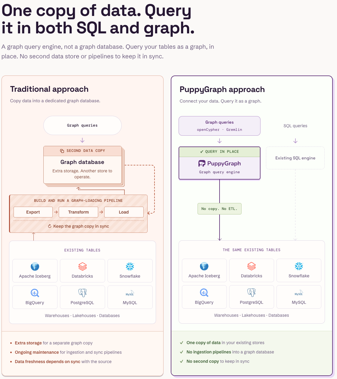
PuppyGraph compiles a graph query into a plan of node and edge operators that runs in its own distributed engine. When reading SQL sources, it issues only simple projection and filter SQL. This execution architecture lets the engine optimize specifically for multi-hop traversals. For a Snowflake dependency investigation, analysts can follow service relationships and extend the model to owning teams while existing SQL reports continue using the same source tables.

Teams can connect through the Snowflake connector or install the Snowflake Native App, which runs PuppyGraph on Snowpark Container Services inside their Snowflake account. The Native App keeps graph compute within that account; source reads still use a Snowflake SQL warehouse. Both arrangements require deliberate data access and schema mappings. Evaluate the graph compute and warehouse reads together when sizing the deployment.

Key components of Snowflake graph

An operational graph solution needs more than an edge table. Its components connect the original records to a repeatable analytical result.

Source records and preparation. Service catalogs, transaction tables, and event records supply the raw material. When relationships arrive in nested arrays, Snowflake's FLATTEN function can turn them into rows. Normalize endpoint types and define which observations qualify as relationships before querying them.

A reusable graph definition. Specify the node identifiers, relationship endpoints, and properties. With SQL, tables, views, and query conventions carry those definitions. An attached graph engine can maintain explicit mappings. Consistent definitions prevent separate analysts from interpreting the same connection differently.

Query compute. Virtual warehouses supply compute for SQL workloads. Separate warehouses can serve reporting and graph-oriented SQL over the same tables. Size them using representative queries, including highly connected starting nodes.

Access and consumers. Snowflake's access-control model governs privileges on source objects. Applications, notebooks, and dashboards consume the results. For an integration, verify the identity used for source reads and the restrictions applied to it; a shared connection does not by itself establish individual users' access boundaries.

Graph data modeling in Snowflake

Model relationships around the question being asked. For dependency analysis, a directed CALLS edge from checkout to payments means checkout calls payments. Ownership is a different relationship and should not silently become another dependency edge.

Choose identifiers at the right scope. A service name may be unique within one environment but collide across production, staging, or separate business units. Use a canonical identifier or a consistent composite key. Resolve aliases before constructing edges, because a traversal cannot recover connections split across inconsistent identities.

Define the edge's grain. One row per observed request is an event graph; one row per caller-callee pair summarizes connectivity. Repeated requests should not accidentally multiply paths when the question concerns distinct dependencies. Keep request counts and observation windows as properties when that aggregation is appropriate.

Snowflake does not enforce primary-key uniqueness or foreign-key references on standard tables. Validate duplicate identifiers, null endpoints, and references to missing services in the data preparation process. Also define when an old observation stops representing an active dependency. Reliable graph results depend on these modeling decisions as much as on query syntax.

For historical investigations, preserve when relationships were valid. Combining yesterday's service ownership with today's calls can produce a technically valid path that never existed in that form. Select a consistent observation interval and retain enough provenance to trace an edge back to its source records. A graph model should make that temporal meaning explicit.

How to build graphs in Snowflake

Build a small, inspectable model before connecting the full inventory. The following example represents one environment at one point in time. Each edge records a distinct caller-callee relationship.

In a Snowflake SQL session with a database, schema, and warehouse selected, create these temporary tables. Run the later queries in the same session:

CREATE TEMP TABLE graph_services (
    service_id VARCHAR NOT NULL,
    owner_team VARCHAR
);

CREATE TEMP TABLE graph_calls (
    edge_id INTEGER NOT NULL,
    caller_id VARCHAR NOT NULL,
    callee_id VARCHAR NOT NULL
);

INSERT INTO graph_services VALUES
    ('checkout', 'commerce'),
    ('payments', 'payments'),
    ('orders', 'commerce'),
    ('identity', 'platform'),
    ('search', 'discovery');

INSERT INTO graph_calls VALUES
    (1, 'checkout', 'payments'),
    (2, 'checkout', 'orders'),
    (3, 'payments', 'identity'),
    (4, 'orders', 'identity');

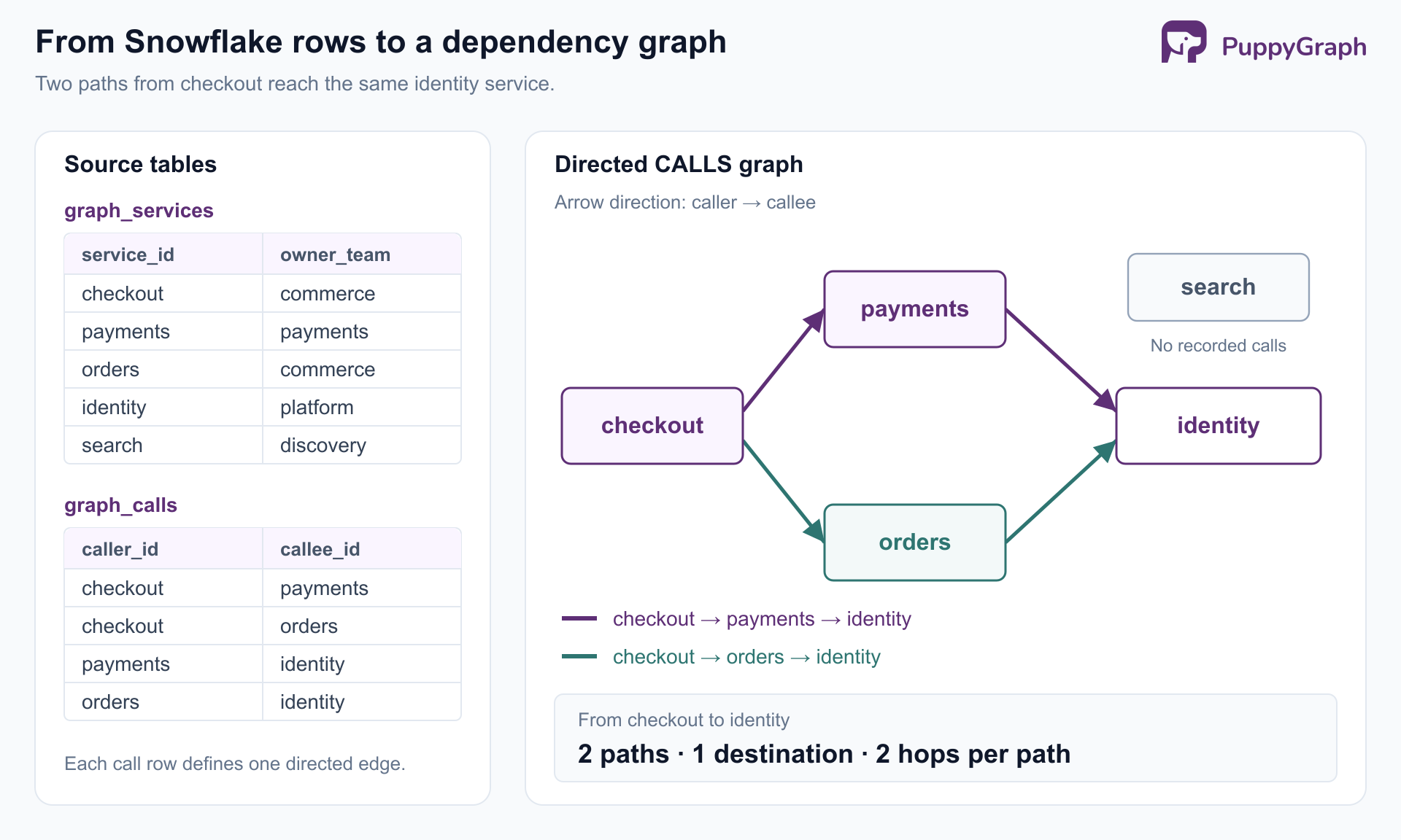
These tables already represent a graph: services are nodes and calls are directed edges. Keeping the service inventory separate preserves services with no recorded connections, such as search. Building the node set only from edge endpoints would omit them.

Before expanding the dataset, check that each service identifier appears once and both endpoints of every edge exist. Validate an expected relationship manually, then check a known absent one. For a lasting deployment, use maintained source tables or views and document how inserts, deletions, and expired observations change the graph. The temporary tables here are only a self-contained example.

If request logs supply the edges, filter them to the intended environment and observation window before reducing them to distinct caller-callee pairs. Keep the original observations available for investigation. An absent edge means no qualifying connection was recorded; incomplete instrumentation or sampling can leave genuine dependencies unseen. In the example, search is isolated by construction. In an operational inventory, investigate missing observations before treating isolation as a fact about the application.

Querying graph data in Snowflake

A direct dependency lookup filters graph_calls by caller_id. A fixed two-hop traversal joins one edge's callee_id to the next edge's caller_id. Snowflake also supports CONNECT BY for hierarchical queries; recursive CTEs provide flexibility when carrying path state or joining additional tables.

This query explores up to four hops from checkout and summarizes the services it reaches:

WITH RECURSIVE paths (service_id, hops, visited) AS (
    SELECT service_id, 0, ARRAY_CONSTRUCT(service_id)
    FROM graph_services
    WHERE service_id = 'checkout'

    UNION ALL

    SELECT e.callee_id,
           p.hops + 1,
           ARRAY_APPEND(p.visited, e.callee_id)
    FROM paths p
    JOIN graph_calls e ON e.caller_id = p.service_id
    WHERE p.hops < 4
      AND NOT ARRAY_CONTAINS(e.callee_id::VARIANT, p.visited)
)
SELECT service_id,
       MIN(hops) AS minimum_hops,
       COUNT(*) AS path_count
FROM paths
WHERE hops > 0
GROUP BY service_id
ORDER BY minimum_hops, service_id;

ARRAY_APPEND records each step. ARRAY_CONTAINS prevents revisiting a service within the same path; its string argument is cast to VARIANT to match the semi-structured array. The hop bound limits expansion independently of that cycle guard.

For this sample, orders and payments each have one path at one hop. Identity has two paths at two hops. The final grouping merges destinations, but it does not remove alternative paths during expansion. minimum_hops describes paths found within the bound, not unrestricted reachability across a larger graph.

Aggregation sits outside recursion because Snowflake's recursive clause restrictions exclude aggregate functions, window functions, and GROUP BY. With larger graphs, filter the eligible edges early and inspect Query Profile for expanding intermediate results and expensive operators. A depth limit prevents unbounded recursion but does not guarantee a small result.

To investigate a failing dependency, anchor the traversal at that service and reverse the edge direction throughout the recursive step. Join the current service to callee_id, return caller_id as the next service, and use that caller in both the path append and the cycle check.

Graph analytics with Snowflake SQL

Graph analytics measures patterns across connections. SQL can calculate useful local measures without enumerating long paths. For example, count each service's distinct outgoing dependencies:

SELECT s.service_id,
       COUNT(DISTINCT e.callee_id) AS outgoing_dependencies
FROM graph_services s
LEFT JOIN graph_calls e ON e.caller_id = s.service_id
GROUP BY s.service_id
ORDER BY outgoing_dependencies DESC, s.service_id;

Checkout has two, orders and payments each have one, and identity and search have zero. The left join preserves zero-degree services; counting the nullable edge endpoint avoids counting an unmatched row as a connection. Join on e.callee_id = s.service_id and count distinct callers to measure incoming dependencies.

Identity illustrates why direction matters: it has no outgoing dependencies in this model but two direct callers. Checkout also depends on it indirectly. Counting distinct reachable callers answers how many services may need investigation; counting paths describes the different dependency chains through which that exposure arises. Neither count measures the number of failed requests.

These measures support practical investigations. Service impact analysis follows dependencies backward from a failing service and joins reachable callers to their owners. Fraud investigation links accounts through devices or payment instruments, then checks timing and other evidence before treating shared infrastructure as suspicious. Supply-chain analysis follows supplier and component relationships to identify products exposed to a disruption. Each use case needs its own edge semantics and business rules.

For graph-wide algorithms such as PageRank or label propagation for community detection, plan the algorithm implementation separately. Their implementations maintain state across iterations and need explicit stopping criteria. Options include a staged computation or a graph engine with the required algorithm; do not assume that support for recursive SQL supplies an entire graph analytics library.

Choose metrics that answer the operational question. High incoming degree can identify a shared dependency, but it does not establish business criticality. Combine connectivity with ownership, service objectives, and observed behavior before turning a graph score into a priority.

Conclusion

Graph analysis over Snowflake starts with stable identities, explicit relationships, and a deliberate execution choice. SQL handles direct connections, bounded traversals, and local measures using warehouse tables. More varied traversal patterns and graph-wide algorithms call for evaluating additional compute and tooling against the actual workload. In either case, path semantics and data quality determine whether the results are useful.

Try the forever-free PuppyGraph Developer Edition and book a demo with the team to see how openCypher and Gremlin queries traverse warehouse and lakehouse tables, with no graph-specific ETL, starting with the service dependencies already stored in Snowflake.