Snowflake Graph Database: Architecture & Features

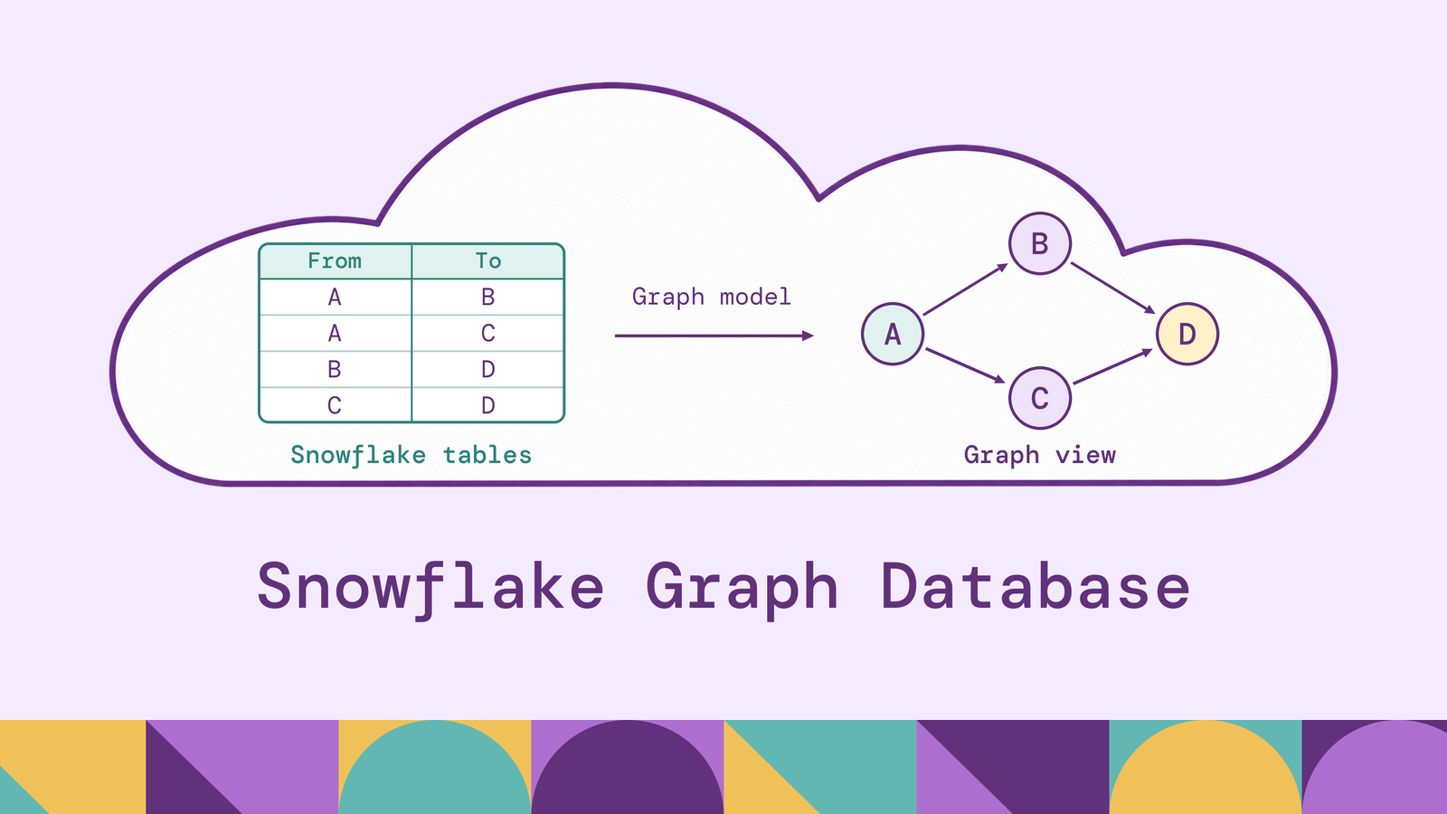
Graph analysis over Snowflake data starts with an architectural choice: how to express multi-hop queries and which engine will execute them. Existing customer records, transactions, and component dependencies can supply the entities and relationships those queries traverse.

This guide explains what a Snowflake graph database means in practice, how to model and query graph data with SQL, and where a dedicated graph query engine fits. A bill-of-materials example shows the difference between storing relationships and traversing them.

What is a Snowflake graph database?

Here, a Snowflake graph database refers to a graph analysis solution built around Snowflake warehouse tables. The phrase describes an architecture or integration rather than a distinct warehouse table type. Snowflake's core architecture provides database storage, SQL compute, and coordinating cloud services. Graph behavior comes from the data model and the queries or additional engine applied to it.

In a property graph, nodes represent entities, edges represent relationships, and properties describe both. For a manufacturer, nodes might represent assemblies and components. A directed edge from an assembly to a component means the assembly requires that component. Quantity belongs on the relationship because different assemblies can require different amounts of the same part.

Snowflake can store these entities and relationships in ordinary tables. SQL joins and recursive queries can follow their connections. An integrated graph engine can expose a graph query language over the data instead. Identify which arrangement a solution uses before comparing its query capabilities, operational requirements, or performance.

How does Snowflake graph database work?

The workflow starts by identifying entities and relationships in source tables. A component table supplies node identifiers and attributes; a bill-of-materials table supplies parent and child identifiers. Each relationship row links two entities through those identifiers.

For a fixed-depth question, a SQL self-join on the relationship table can find a component's dependencies and their dependencies. When depth varies, recursive common table expressions repeat a traversal step: an anchor selects the starting entities, and a recursive clause expands the current results to the next connected entities. Results accumulate until expansion produces no rows or a query condition stops it.

The direction matters. Following assembly-to-component edges finds required parts. Following those edges backward finds assemblies potentially affected by a component shortage. Neither direction automatically answers how much inventory is needed; that requires quantity calculations and business rules.

Define the answer before choosing the traversal. A list of reachable components, every dependency path, and the shortest path to each component are different outputs, even when they use the same tables.

Snowflake graph database architecture

For standard Snowflake tables, the storage layer organizes data in a compressed columnar format. A virtual warehouse executes SQL over those tables. Cloud services coordinate authentication, metadata, and query planning. Graph queries expressed in SQL use these same layers.

Three arrangements are useful to distinguish:

These are architectural patterns, not performance rankings. A small hierarchy may work well with recursive SQL. An application that repeatedly explores changing relationship patterns may benefit from a graph query interface. A separate graph store can serve workloads that justify independently managed graph storage.

For any integration, trace the complete query path. A graph-shaped API alone does not establish where traversal executes: the integration might compute graph operations itself or translate them into SQL. Likewise, a connector does not imply direct access to Snowflake's internal storage files. Separate storage location, execution location, and deployment location when reviewing the design.

Key features of Snowflake graph database

The relevant features are Snowflake capabilities that support graph workloads, together with graph functionality supplied by an integration.

Recursive SQL. Snowflake supports recursive CTEs and CONNECT BY for hierarchical queries. Recursive CTEs allow additional joins and explicit path state, which is useful when a traversal needs attributes from several tables.

Flexible source data. Snowflake supports semi-structured data, including JSON stored in VARIANT columns. FLATTEN can turn nested arrays into rows for relationship modeling. Extract identifiers into consistently typed columns before using them as graph endpoints.

Independent compute resources. Virtual warehouses provide configurable compute for SQL workloads. Teams can allocate separate warehouses to reporting and relationship analysis while accessing the same tables. Warehouse sizing still needs to reflect the actual query workload.

Source governance. Row access policies filter visible rows, while Dynamic Data Masking controls exposed column values. Both require Enterprise Edition or higher. With an external application, test the identity and session context under which its reads execute.

These features provide storage, processing, and governance foundations. The chosen graph integration determines its supported graph language, algorithms, and visualization tools.

Graph data modeling in Snowflake

Start with one concrete question, such as which components an assembly depends on indirectly. Model only the entities and relationships needed to answer it before expanding to suppliers, shipments, and inventory.

Choose stable identities. A component identifier must identify the same component across all relevant tables. If identifiers are unique only within a tenant or source system, include that scope in the identity. Joining unrelated records that share a local identifier creates false paths.

Make edges explicit. Store the parent identifier, child identifier, and relationship attributes together. Define direction once: parent_component_id → child_component_id means requires. A separate edge identifier distinguishes multiple records between the same endpoints when those records represent different events or contracts.

Preserve time and provenance. A current bill of materials and a historical one answer different questions. Keep revision or validity information when the analysis requires it, and retain enough source information to explain a returned path. Filter each relationship to the intended time context.

Validate the model. Snowflake does not enforce primary-key uniqueness or foreign-key references on standard tables. Check for duplicate node identifiers and edges whose endpoints are missing. A declared constraint alone does not establish graph integrity.

Keep the logical graph separate from the physical table layout. A purchase-order line can supply an edge between a supplier and a component even if nobody named that table an edge table. Preserve the business identifiers and define which records qualify for each relationship. This lets the graph reuse existing warehouse models without forcing every source into one generic node table.

The graph model is a contract about meaning. A shared supplier indicates a connection, but it does not by itself prove a supply-chain risk. Interpretation depends on the relationship's semantics and the evidence stored with it.

How to create graph data in Snowflake

The following example creates a small dependency graph. Use a scratch schema with a selected warehouse and permission to create tables. Run the setup once with unused table names.

Create the nodes and edges. The assembly requires a pump and a valve; both require a gasket. These are ordinary Snowflake tables created with CREATE TABLE and populated with INSERT:

CREATE TABLE graph_components (
    component_id VARCHAR NOT NULL,
    component_name VARCHAR NOT NULL
);

CREATE TABLE graph_dependencies (
    edge_id VARCHAR NOT NULL,
    parent_component_id VARCHAR NOT NULL,
    child_component_id VARCHAR NOT NULL,
    quantity NUMBER(10, 0) NOT NULL
);

INSERT INTO graph_components VALUES
    ('A', 'Assembly'),
    ('B', 'Pump'),
    ('C', 'Valve'),
    ('D', 'Gasket');

INSERT INTO graph_dependencies VALUES
    ('e1', 'A', 'B', 1),
    ('e2', 'A', 'C', 1),
    ('e3', 'B', 'D', 2),
    ('e4', 'C', 'D', 1);

Check the endpoints. This query should return no rows. It catches edges that reference components absent from the node table:

SELECT e.edge_id
FROM graph_dependencies e
LEFT JOIN graph_components p
    ON p.component_id = e.parent_component_id
LEFT JOIN graph_components c
    ON c.component_id = e.child_component_id
WHERE p.component_id IS NULL OR c.component_id IS NULL;

Also check identifier uniqueness before running a larger dataset. Duplicate rows can multiply traversal results even when every endpoint exists.

Traverse the dependencies. This query starts at assembly A, follows up to four edges, and tracks visited identifiers to avoid revisiting a component within a path:

WITH RECURSIVE dependency_walk (component_id, depth, path) AS (
    SELECT component_id, 0, ARRAY_CONSTRUCT(component_id)
    FROM graph_components
    WHERE component_id = 'A'

    UNION ALL

    SELECT e.child_component_id,
           w.depth + 1,
           ARRAY_APPEND(w.path, e.child_component_id)
    FROM dependency_walk w
    JOIN graph_dependencies e
        ON e.parent_component_id = w.component_id
    WHERE w.depth < 4
      AND NOT ARRAY_CONTAINS(e.child_component_id::VARIANT, w.path)
)
SELECT w.component_id, c.component_name, MIN(w.depth) AS min_hops
FROM dependency_walk w
JOIN graph_components c ON c.component_id = w.component_id
WHERE w.depth > 0
GROUP BY w.component_id, c.component_name
ORDER BY min_hops, w.component_id;

ARRAY_APPEND extends the path. ARRAY_CONTAINS checks whether the next identifier already appears in it; the string is cast to VARIANT for comparison with the semi-structured array.

Expected output:

The gasket is reachable through two paths but appears once because the final aggregation groups by component. MIN_HOPS reports the shortest distance found within the four-hop search boundary. This query answers reachability; calculating required gasket quantities would require multiplying quantities along paths and summing the relevant contributions.

The grouping happens after recursion because Snowflake's recursive clause restrictions exclude aggregate functions and GROUP BY. The path guard prevents cycles within each path, but does not eliminate alternative paths to the same component during expansion.

Benefits of Snowflake for graph database

The main benefit is reuse of data and analytical work already maintained in Snowflake. A dependency analysis can use the same component identifiers, supplier records, and inventory attributes as operational reports. Teams can validate a relationship result against the underlying rows without reconciling a separately curated dataset.

This supports concrete applications. Supply-chain teams can trace which assemblies depend on a recalled component. Fraud investigators can examine accounts connected through shared devices or payment instruments. Data teams can follow dependencies from a changed source column to downstream assets, provided those lineage relationships have been collected. In each case, the graph question connects records across steps, while ordinary reporting supplies counts, amounts, and business context.

PuppyGraph is the first and only zero-ETL graph query engine that lets teams query existing relational data as a graph without building a separate graph ingestion pipeline. For Snowflake, teams define a graph schema over existing tables and query it with openCypher or Gremlin. The schema supplies a semantic model of components, suppliers, and dependencies; the default direct-query path requires no persistent duplicate dataset.

PuppyGraph compiles a graph query into a plan of node and edge operators that runs in its own distributed engine. When reading SQL sources, it issues only simple projection and filter SQL. This execution architecture lets it optimize specifically for multi-hop traversals. For the component example, analysts can explore dependencies and extend the model to supplier relationships while Snowflake continues serving inventory reports from the same source tables.

Teams can use the Snowflake connector or deploy the Snowflake Native App, which runs PuppyGraph on Snowpark Container Services inside their Snowflake account. Both approaches require granting access to the intended data and defining the graph mappings. The Native App changes where the engine is deployed; graph traversal still executes in PuppyGraph, and source reads still use a Snowflake SQL warehouse. This makes the integration a concrete option for adding relationship analysis to an existing warehouse workflow.

Snowflake graph database limitations

Traversal growth. A dependency tree with limited branching is different from a densely connected network. The example preserves alternative paths, so intermediate rows can grow much faster than the number of unique nodes. Filter the starting population and relationship types, set a justified depth boundary, and evaluate representative high-degree entities.

SQL maintenance. Recursive SQL is useful, but complex path conditions and changing relationship patterns make queries harder to review. Snowflake's recursive clause excludes aggregates, window functions, and DISTINCT. Designs that need deduplication or iterative global state may require staged processing or a graph engine.

Compute and integration costs. Keeping data in Snowflake avoids a required graph copy only for architectures that actually query the source. Those reads still consume warehouse resources. An attached engine adds its own compute, while a copied graph adds storage and synchronization work. Compare total operating cost against the query workload.

Freshness and access boundaries. Direct querying does not repair stale upstream ingestion or incomplete entity resolution. A copied or cached graph also needs a defined refresh policy. For integrations, verify which identity reaches Snowflake and whether each user's required restrictions are applied; connecting one shared service account does not automatically establish per-user isolation.

Choose the design using actual questions and data distributions. Table size alone does not predict traversal cost, and successful execution on a small sample does not establish acceptable latency for an interactive application.

Conclusion

A Snowflake graph database architecture combines a relationship model with a deliberate choice of query engine. SQL is a practical starting point for bounded dependency analysis. A graph engine becomes useful when reusable graph semantics and more varied traversals matter to the workload. Stable identities, explicit edge direction, and controlled expansion remain necessary in either design.

Try the forever-free PuppyGraph Developer Edition and book a demo with the team to see how openCypher and Gremlin queries traverse warehouse and lakehouse tables, with no graph-specific ETL, starting with the dependency relationships already stored in Snowflake.