Predicate Pushdown: How It Works?

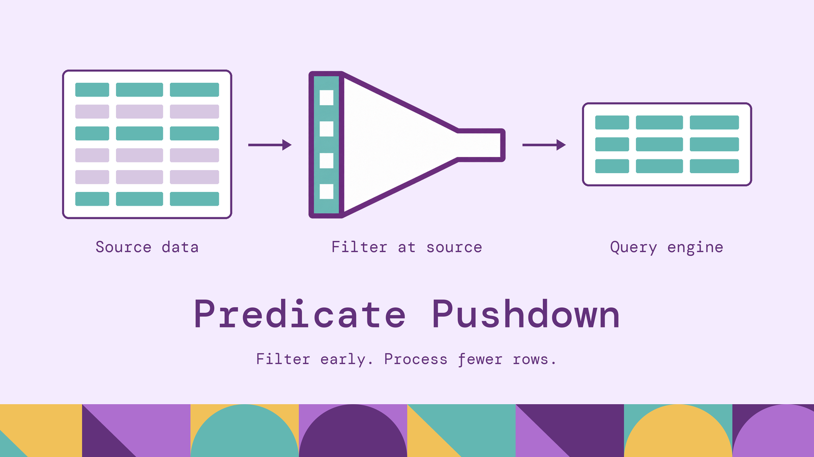
A query that returns a handful of rows can still read most of a table. The difference depends on where its filters run and whether the storage layer can exclude data before reading it. Predicate pushdown moves filtering toward the data source, reducing the work that reaches joins, aggregations, and network exchanges.

This guide explains how predicate pushdown works in SQL databases, Apache Spark, and data lakes, how to write queries that support it, and how to distinguish a pushed filter from a measurable reduction in work.

What is predicate pushdown?

Predicate pushdown is a query optimization that moves a filtering condition closer to the operation that reads its input, while preserving the query's result. A predicate is a condition such as status = 'paid' or order_date >= DATE '2026-01-01'. In a SQL WHERE clause, only rows for which the condition evaluates to true survive.

The word down refers to the query plan. Scans typically appear below joins and aggregations. Moving a filter down the plan can eliminate rows before those later operators process them. Across a connector boundary, pushdown means asking the source to evaluate a supported condition. Trino's pushdown documentation describes this delegation and its dependence on connector capabilities.

Pushdown does not guarantee that storage reads decrease. A database can scan every row, filter locally, and return only the matches. That saves transfer and downstream processing. Avoiding reads requires an access mechanism, such as an index or usable file statistics, that can exclude data without examining every row.

How does predicate pushdown work?

Consider an orders table with order_id, customer_id, order_date, and amount, joined to customers with customer_id and region:

SELECT o.order_id, o.amount, c.region
FROM orders AS o
JOIN customers AS c
  ON o.customer_id = c.customer_id
WHERE o.order_date >= DATE '2026-01-01'
  AND o.order_date < DATE '2026-02-01'
  AND c.region = 'EMEA';

The date predicates refer only to orders; the region predicate refers only to customers. For this inner join, the optimizer can filter each input before joining. Conceptually, the plan reads January orders and EMEA customers, then matches their customer identifiers. Writing WHERE after JOIN does not require the database to build the complete join result first.

The optimizer next determines which conditions the scan or connector can handle. A SQL source might receive a date-bounded query. A Parquet reader might receive the same bounds and inspect row-group statistics. Conditions that cannot be handled completely at that level remain as residual filters for later evaluation.

Suppose a Parquet row group's maximum order_date is December 31, 2025. It cannot contain January 2026 orders and can be skipped. A row group spanning December through February remains a candidate. Its bounds do not establish which individual rows match, so row-level filtering may still be needed. Spark's filter pushdown interface explicitly recognizes pushed filters that require evaluation again after scanning.

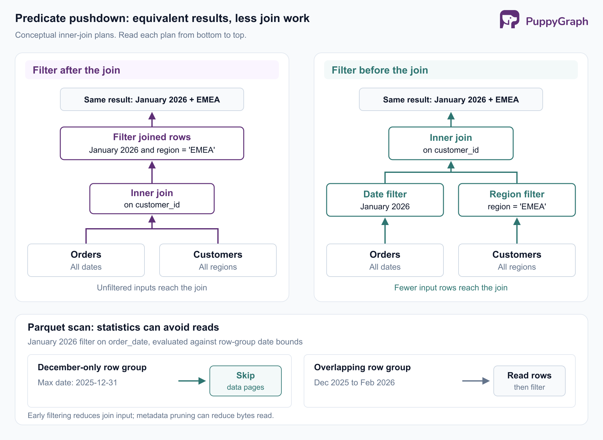
Every movement must preserve semantics. Moving a right-table condition from WHERE into a left join's ON clause can change which unmatched rows survive, as PostgreSQL's join examples demonstrate. Pushdown is a valid plan transformation, not permission to relocate clauses arbitrarily.

Why is predicate pushdown important

Analytical queries often select a narrow slice of a much larger dataset: one customer's transactions, one month's orders, or incidents for a particular service. Filtering late makes the infrastructure handle records that cannot contribute to the answer.

In a distributed query, that unnecessary work can cross several boundaries. Rows travel from storage to workers, enter intermediate batches, and may be shuffled between workers before a join. A selective filter applied before those steps can reduce several costs at once. Adding workers increases capacity, but does not remove the underlying waste.

The distinction matters particularly when compute and storage are separate. A query engine reading a remote database pays for transferring the returned rows. An engine reading object storage also depends on how effectively metadata identifies relevant files and regions within them. The same SQL predicate can therefore have very different consequences across storage layouts.

This makes predicate pushdown a useful starting point for diagnosis. Before increasing memory or cluster size, determine whether irrelevant data reaches the expensive operators. The answer helps distinguish a query-planning problem from a storage-layout problem or a workload that legitimately needs a broad scan.

Types of predicate pushdown

The term covers several execution layers. These mechanisms can work together within one query; they are not mutually exclusive modes.

SQL databases also optimize across query blocks. MySQL's derived-condition pushdown can move an outer filter into an eligible subquery. A condition on a grouping key may move before aggregation; a condition on an aggregate result still needs aggregation before evaluation.

For data lakes, pruning is the data-skipping mechanism enabled by suitable predicates. Apache Iceberg's scan planning uses partition metadata and column-level bounds to eliminate candidate files. A reader can subsequently apply finer filtering within the files that remain.

Projection pushdown is complementary: it limits the columns read or returned. Predicate pushdown restricts rows. Selecting only order_id and amount can reduce column reads, while the date condition restricts eligible records. Columns needed to evaluate filters or joins still have to be available, even when they do not appear in the final output.

Benefits of predicate pushdown for query performance

Lower scan I/O. When metadata excludes a file or row group, the reader can avoid its data pages. This matters when storage access dominates execution time. The benefit depends on the distribution of values: a narrow date query cannot skip much if every row group's date range spans the entire year.

Less network traffic. A remote database that evaluates the predicate can return fewer rows to the calling engine. Filtering before a distributed exchange can also reduce shuffle traffic. These are separate effects, so inspect both source transfer and communication between workers when evaluating a federated query.

Smaller intermediate workloads. Fewer rows entering joins and sorts means less processing. Filtering a hash join's build input can reduce its hash table and the chance of spilling to disk. Filtering an aggregate's input reduces rows processed, although memory use also depends on the number of groups that remain. Early filtering does not shrink every operator's state proportionally.

These effects can lower query cost or improve shared-cluster throughput, but the billing model and actual bottleneck determine the outcome. A predicate matching most rows offers little reduction. An expensive expression delegated to a busy source can also shift the bottleneck rather than remove it; Spark's JDBC documentation acknowledges cases where filtering in Spark can be faster.

Measure the avoided work. A pushed predicate is useful evidence about execution, but it is not a performance result by itself.

How to implement predicate pushdown

Most engines apply eligible transformations automatically. The practical work is making filters understandable to the optimizer, using a capable source, and choosing a layout that allows selective reads.

Use direct comparisons with compatible types. For a SQL DATE column, a range expresses the January restriction directly:

WHERE order_date >= DATE '2026-01-01'
  AND order_date < DATE '2026-02-01'

This exposes column bounds without requiring the source to translate an expression such as EXTRACT(MONTH FROM order_date) = 1. The year boundary also makes the intended period explicit. Function-wrapped columns are not universally unoptimizable, but support depends on the engine, indexes, and connector. Preserve timezone semantics when adapting date ranges to timestamp columns.

Keep Spark filters in structured expressions. With an existing SparkSession named spark, the following reads a Parquet dataset whose order_date column has type DATE. Replace the example path with your dataset location:

spark.conf.set("spark.sql.parquet.filterPushdown", "true")

orders = spark.read.parquet("/data/orders")
january_orders = (
    orders
    .where("order_date >= DATE '2026-01-01' "
           "AND order_date < DATE '2026-02-01'")
    .select("order_id", "amount")
)

Spark documents Parquet filter pushdown as enabled by default; the setting makes the example explicit. Native column expressions expose the condition to planning. A Python UDF implementing the same comparison generally cannot be translated into a Parquet reader predicate. Apply supported restrictions before custom processing when the result remains equivalent.

For JDBC reads, Spark exposes a separate pushDownPredicate reader option, also enabled by default. Check the relevant connector instead of assuming the Parquet setting controls every source. An enabled option permits supported pushdown; it does not make every expression translatable.

Align storage layout with recurring filters. Date partitioning can make time-bounded queries selective at the file level. Sorting or clustering on frequently filtered columns can make min/max ranges more useful within the selected data. Iceberg's hidden partitioning derives partition restrictions from supported predicates on source columns, so queries need not manually reproduce a separate partition-key calculation.

For example, placing records with nearby order dates together produces narrower date bounds than randomly distributing dates across files. This effect comes from storage layout. Choose partition granularity against the workload and file sizes; creating excessive small partitions introduces metadata and file-management overhead.

The same filtering principles apply when the question follows relationships across tables. An investigation might start with a subset of customers, follow their orders, and identify shared suppliers. PuppyGraph lets you define a graph schema over existing tables and query those relationships using openCypher and Gremlin. Its Iceberg tutorial shows this mapping while the source data remains in the lakehouse, with no graph-specific ETL.

PuppyGraph compiles a graph query into a plan of node and edge operators that runs in its own distributed engine. When reading SQL stores, it issues only simple projection and filter SQL. This execution architecture lets the engine optimize specifically for multi-hop traversals. It also uses predicate pushdown and min/max statistics to reduce data scanned. Source filtering reduces the data feeding that work, while the traversal executes inside PuppyGraph.

How to verify predicate pushdown using query plans

Verification has two parts: locate the filter in the plan, then measure the work performed. A short runtime alone proves neither where filtering occurred nor why the query was fast.

For the Spark DataFrame above, inspect the physical plan and scan details with explain:

january_orders.explain(mode="formatted")

In a typical Spark Parquet file-scan plan, look for these fields:

• PushedFilters identifies predicates passed toward the data source, such as date comparisons and null checks.
• PartitionFilters identifies restrictions used for partition selection. If order_date is a partition column, its conditions may appear here instead of under PushedFilters.
• ReadSchema identifies the physical columns requested from the files, including columns needed for filtering.

Labels and presentation vary across connectors and scan implementations. Read them together: a narrow read schema demonstrates column selection, while pushed filters show predicate delegation. Neither field reports the bytes actually avoided.

A separate Filter above the scan can be correct. Row-group pruning retains groups that might match, and Spark may still need to evaluate the predicate on their rows. Removing every visible filter operator is not the objective.

Then execute a representative workload that consumes the filtered data. Use the Spark UI's SQL and stage metrics to inspect scan time, input bytes, output rows, and shuffle volume. For a controlled comparison, rebuild the DataFrame after changing pushdown settings and keep data, projection, cache conditions, and compute resources comparable. A small preview may stop early and does not represent a complete scan.

In PostgreSQL, inspect the equivalent date filter with:

EXPLAIN (ANALYZE, BUFFERS)
SELECT order_id, amount
FROM orders
WHERE order_date >= DATE '2026-01-01'
  AND order_date < DATE '2026-02-01';

ANALYZE executes this query. An Index Cond shows a condition used in index access. A Filter attached to a sequential scan rejects rows after reading them; it does not establish that table pages were skipped. PostgreSQL's EXPLAIN guide distinguishes these operations and explains actual rows, removed rows, and buffer activity.

When pushdown appears in the plan but reads remain high, inspect selectivity and data layout. When a supported filter is absent, inspect casts, UDFs, connector support, and execution boundaries. Those are different problems and call for different changes.

Conclusion

Predicate pushdown reduces unnecessary work by moving eligible filters toward the data they restrict. Its value depends on where filtering happens, what the source can execute, and whether indexes or metadata can avoid reads. Write clear predicates, design storage around recurring access patterns, and confirm the result with plans and runtime metrics.

Try the forever-free PuppyGraph Developer Edition and book a demo with the team to see how openCypher and Gremlin queries follow relationships across warehouse and lakehouse tables, with no graph-specific ETL, using source filtering to reduce the input to graph analysis.