What Is Graph Data Structure?

Most of the data you care about is about relationships. A customer buys a product. A flight connects to another flight. A service calls another service. Arrays and trees struggle to model that world cleanly, and that's exactly the gap the graph data structure fills.

This guide walks through what a graph data structure is, how it works in practice, the different types you'll encounter, how graphs get stored in memory, and why graph thinking keeps showing up in modern data systems. By the end, you'll know when a graph is the right tool and how to reason about performance when you reach for it.

What Is a Graph Data Structure?

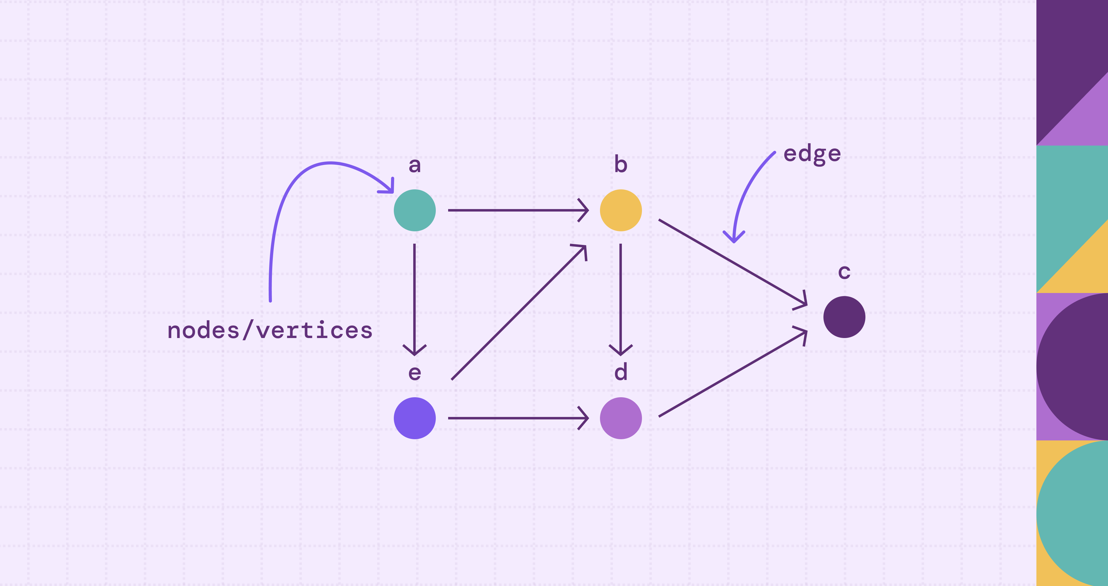
A graph data structure is a non-linear collection of nodes (also called vertices) connected by edges that represent relationships between them. Unlike arrays or linked lists, a graph has no inherent ordering and typically no single root (unless you're modeling a tree or DAG). Any node can connect to any number of other nodes, and the connections themselves can carry meaning.

Formally, a graph is a pair \(G = (V, E)\) where \(V\) is a set of vertices and \(E\) is a set of edges. In an undirected graph, each edge is an unordered pair of vertices; in a directed graph, each edge is an ordered pair. As an abstract data type in computer science, a graph supports operations like adding vertices, adding edges, and querying whether two nodes are connected. Everything else (direction, weight, labels, properties) is an elaboration on top of that core.

The easiest way to picture a graph is to think about anything you'd draw with circles and lines. A subway map is a graph. Stations are nodes, tracks are edges, and travel time on each track is an edge weight. Google Maps models road intersections as vertices and road segments as weighted edges to compute the shortest path between two locations. A social network is a graph, with people as nodes and friendships as edges. The dependency tree of your package.json is a graph (technically a directed acyclic graph, or DAG, with a root node at the top-level package).

Graphs show up everywhere because real systems are full of many-to-many relationships that don't flatten nicely into rows and columns. A customer can buy thousands of products. A product can be bought by thousands of customers. Trying to answer "show me customers who bought what my top customers bought" in pure SQL often requires multiple self-joins. In a graph, it becomes a short multi-hop traversal.

For a deeper look at the core components, see our guide on nodes and edges in graph theory.

How Does Graph Data Structure Work?

A graph works by letting you move between nodes along edges. That movement is called traversal, and almost every useful thing you do with a graph boils down to traversing it in some smart way.

Let's ground this in a concrete example. Imagine five people on a small social network: Alice, Ben, Carla, Dev, and Eve. Alice knows Ben and Carla. Ben knows Dev. Carla knows Dev and Eve. You can draw this as five nodes with edges between the people who know each other.

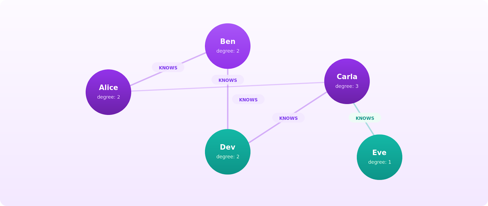
Now ask a question: who are Alice's friends-of-friends? You start at Alice, follow her edges to Ben and Carla, and then follow their edges outward. Ben points you to Dev. Carla points you to Dev and Eve. The answer is Dev and Eve, reached in exactly two hops. That's a traversal, and it's the kind of query graphs are built for.

To describe traversals precisely, graph theory gives you a small vocabulary:

• Adjacency: two nodes are adjacent if an edge connects them. Alice and Ben are adjacent vertices, which also makes them neighboring vertices.
• Degree: the number of edges touching a node. Alice has a degree 2.
• Path: a sequence of edges you follow from one node to another. Alice -> Carla-> Eve is a path of length 2.
• Cycle: a path that starts and ends at the same vertex without repeating edges.
• Connected components: sets of nodes where every node can reach every other node through some path. A connected graph has exactly one component.

The two foundational graph traversal algorithms are breadth-first search (BFS), which explores all adjacent nodes at the current depth level before going deeper, and depth-first search (DFS), which follows one branch to its end before backing up. Both run in \(O(V + E)\) time on an adjacency list representation, which is the theoretical floor for visiting every node and edge once. From these two, you build up to shortest path algorithms like Dijkstra's, minimum spanning tree algorithms like Prim's and Kruskal's, ranking algorithms like PageRank (originally designed to rank web pages), and clustering algorithms that detect communities. For a broader tour, see our rundown of graph traversal algorithms and the landscape of graph algorithms that sit on top of them.

Types of Graphs in Data Structures

"Graph" isn't one thing. It's a family of shapes, and the shape you pick changes what questions you can ask and how efficiently you can answer them. 

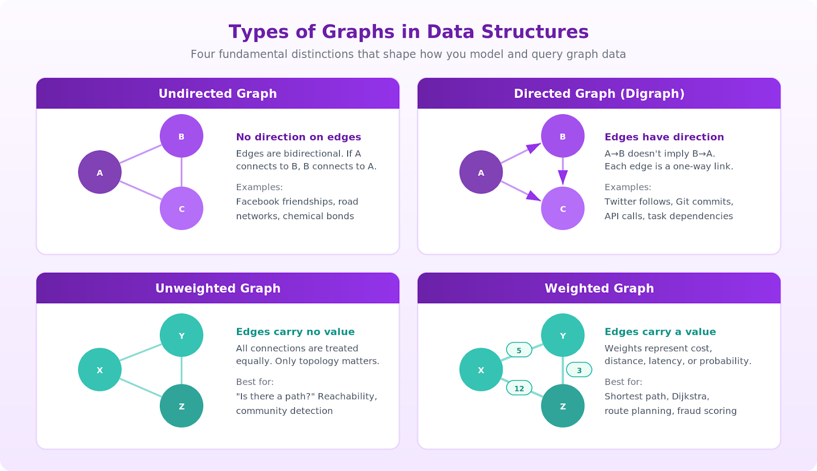
These are the distinctions you'll meet most often:

A few of these deserve a closer look because they change your algorithm choices.

Directed acyclic graphs (DAGs) show up whenever you need to model dependencies. Task schedulers, build systems, Git commit histories, and component trees are all DAGs. Because they have no cycles, you can topologically sort them, processing each node only after all its dependencies are resolved.

In a directed graph, each vertex has both incoming edges (edges pointing to it) and outgoing edges (edges pointing away from it). This distinction matters for algorithms like topological sorting, where you process nodes with zero incoming edges first.

Weighted graphs unlock shortest path questions. The weight might represent distance, latency, cost, probability, or any numeric signal. Change the weight definition, and the "shortest path" becomes a different thing: the cheapest flight across a transportation network, the lowest-latency service route, the most likely fraud chain.

Property graphs extend the basic model by letting nodes and edges carry arbitrary key-value attributes. This is the model used by most modern property graph systems, including those supporting openCypher and Apache TinkerPop Gremlin, because real-world entities have more than just an ID and a type. A Person node might carry name, age, and signup_date. A KNOWS edge might carry since and strength. For a detailed walkthrough of modeling decisions, see graph data modeling.

Graph Representation Methods

Once you pick a graph type, you have to decide how to store it. The representation you choose determines how much memory the graph uses and how fast each operation runs. There are three representations you'll see constantly.

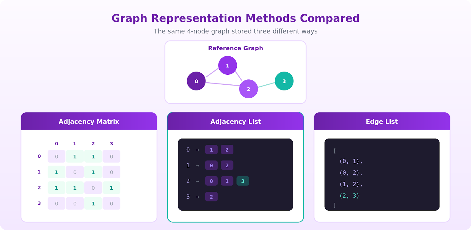
Adjacency matrix. The adjacency matrix representation uses a \(V \times V\) grid where entry \([i][j]\) is 1 (or the edge weight) if there's an edge from node \(i\) to node \(j\), and \(0\) otherwise.

Checking whether an edge exists between two vertices is \(O(1)\). Iterating over a node's neighbors is \(O(V)\) because you have to walk the whole row. Space is \(O(V^2)\), which scales with the number of vertices squared. For sparse graphs, that's brutal: a million-node social network stored as a matrix would need a trillion cells, most of them zero.

Adjacency list. The adjacency list representation uses an array (or hash map) where each node points to a list of its neighboring vertices.

Space is \(O(V + E)\), which is the right answer for almost every real graph because real graphs are sparse. Iterating over a node's neighbors is \(O(degree)\). The trade-off: checking whether a specific pair \((u, v)\) is connected costs \(O(degree(u))\) instead of constant time.

Edge list. A flat list of \((u, v)\) pairs (plus weight if the graph is weighted).

Space is \(O(E)\), and it's the most compact format for transmission and bulk import. It's poor for traversal because you have to scan the entire list to find a node's neighbors, but it's what you'll hand to a batch algorithm like union-find or export from a database.

The practical rule of thumb is to use an adjacency list by default, reach for an adjacency matrix only when the graph is dense or small enough that \(V^2\) memory is fine, and treat edge lists as an interchange format rather than an in-memory working structure.

Benefits of Graph Data Structures

Graphs earn their place in the toolbox because they match the shape of certain problems perfectly. Four benefits stand out.

They model relationships as first-class citizens. In a relational schema, a relationship is something you fake with a foreign key and recover with a JOIN. In a graph, the relationship is an actual edge with its own properties, and walking across it costs the same as reading a column. Multi-hop questions ("find accounts that share a device with an account flagged for fraud last week") go from five-JOIN nightmares to short traversals.

They're flexible under schema change. Adding a new relationship type doesn't require a migration. You just start writing edges with a new label. This is why graphs tend to win in domains where the data model evolves constantly: fraud rings change tactics, product catalogs grow new categories, and org charts reshuffle.

They're efficient for traversal-shaped workloads. Once your query pattern is "start here, walk out N steps, collect something," a graph representation can significantly outperform a relational one, especially at depth 3 or more. Relational queries tend to get increasingly expensive as joins stack on highly connected data, while graph traversals are typically proportional to the portion of the graph actually explored.

They map directly to real-world systems. Social networks, supply chains, IT infrastructure, recommendation systems, knowledge graphs, identity resolution, and cyber-attack paths are all natively graph-shaped. Trying to reason about them as tables is fighting the data model.

That said, graphs are not always the right choice. For simple aggregations, OLAP-style analytics, or workloads with minimal relationship traversal, columnar databases often outperform graph systems. The sweet spot for graphs is when the relationships themselves are what you're querying.

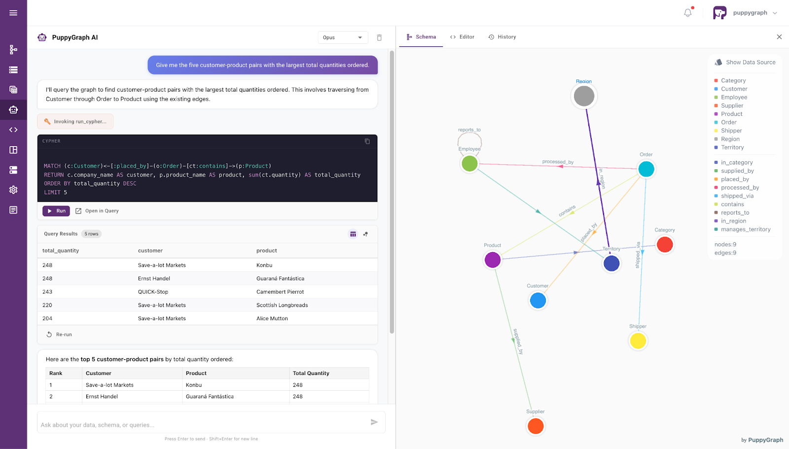
The catch is that adopting a graph often means migrating to a dedicated graph database, which is a heavy lift when your data already lives in Postgres, Snowflake, Databricks, BigQuery, or an Iceberg lakehouse. This is where PuppyGraph fits in. PuppyGraph is a zero-ETL graph query engine that maps existing SQL tables to a graph model and lets you run openCypher and Gremlin queries against them directly, without duplicating or moving data into a separate graph database. You get the traversal benefits of a graph without duplicating your warehouse.

Conclusion

The graph data structure is the right abstraction whenever relationships carry as much meaning as the entities themselves. You've seen the core components (nodes and edges), the common types (directed, weighted, DAG, property graph), the three representations you'll use in practice (adjacency matrix, adjacency list, edge list), and why graphs keep winning in domains full of many-to-many connections.

The next step depends on what you're building. If you're studying algorithms, implement BFS and DFS from scratch over an adjacency list and then layer Dijkstra's on top. If you're a practitioner with data that's already graph-shaped but stuck in SQL, you don't have to choose between rebuilding your stack and giving up on graph queries. Try PuppyGraph's free developer edition and point it at your existing warehouse to see your data as a graph in minutes, or book a demo with our team of graph experts to see it in action.