Nodes and Edges in Graph Theory

In graph theory, a graph consists of a set of nodes and a set of edges, where each edge connects a pair of nodes. Each node represents an entity, and each edge represents a relationship between two entities. Graphs provide a powerful abstraction for modeling real-world systems and seeing how everything connects. A cybersecurity graph might map how system-critical infrastructure touches public-facing assets, while a social network might show how users are connected to one another. 

In this blog, we look at the fundamentals of nodes and edges, how graphs represent relationships, the main graph types, real-world applications, and how to build and query them using modern graph tools such as PuppyGraph.

Introduction to Nodes and Edges in Graph Theory

Let’s examine the basic building blocks of our graphs. Nodes, also known as vertices, represent a “thing” in your system. Edges, also known as links, represent the connections between these entities.

Edges can be directed or undirected.

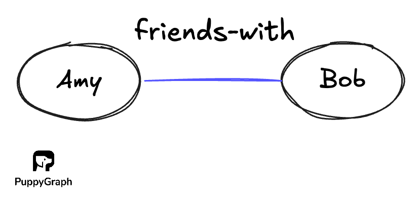
Undirected edges implies a symmetric relation, where if there is a relation from Node A to Node B, there is an equal relation from Node B to Node A, where \((a,b) = (b,a)\). As such, undirected edges are often written as set {a, b} to emphasize that the order does not matter. An example of such a relationship would be “friends-with”.

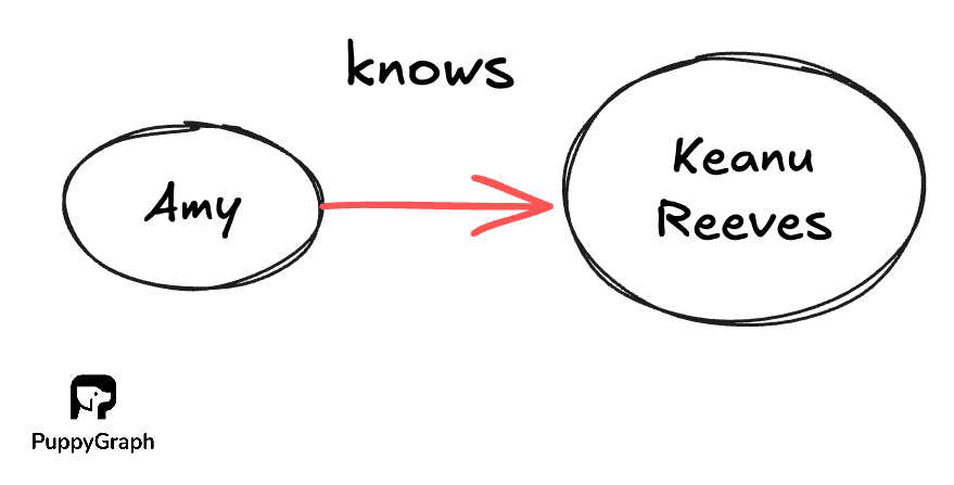
In contrast, directed edges means that the relationship isn’t necessarily reciprocated. For example, if Amy “knows” of the famous celebrity Keanu Reeves, Keanu Reeves need not “know” who Amy is. 

What is a Nodes and Edges Graph?

Formally, a graph is a pair \(G = (V, E)\):

• V, a nonempty set of unique objects, points, or nodes
• E, a set of pairs of nodes that represent connections.

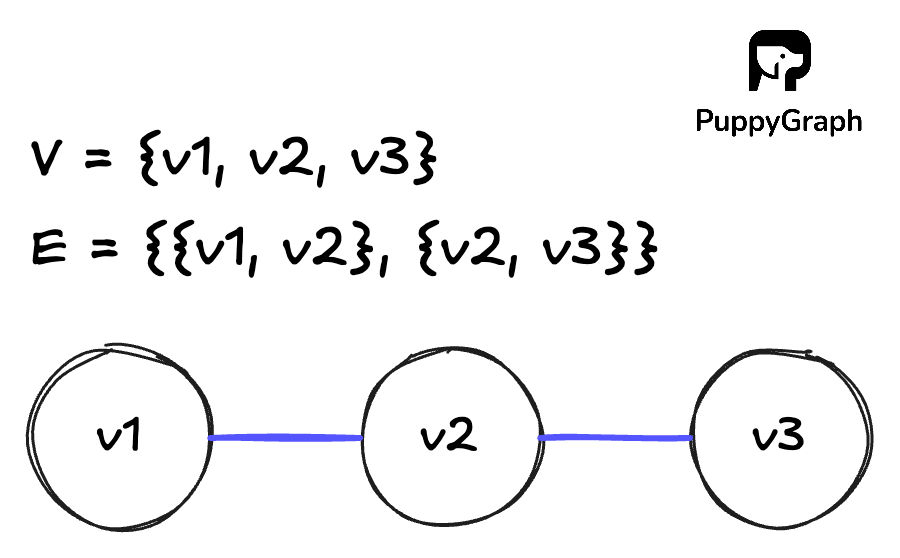
For an undirected graph G, we can define it with set notation as follows:

\[V = \{v1, v2, v3\}\]

\[E = \{\{v1, v2\}, \{v2, v3\}\}\]

This notation can look abstract at first. A more intuitive way to understand it is with a node link diagram. Nodes are drawn as points or circles, and edges are drawn as lines connecting those nodes. The same formal definition \(G = (V, E)\) simply tells you which circles exist and which pairs of circles should be connected by lines.

We can represent the graph in two ways: adjacency lists and adjacency matrices. 

Adjacency List

An adjacency list is a collection of lists, where each node keeps a list of its neighbors. For the undirected graph G that we defined earlier:

Adjacency lists have a space complexity of \(O(V + E)\) since you only store edges that actually exist, helping to save space. This makes adjacency lists a natural fit for sparse graphs, where the number of edges is relatively small compared to the maximum possible number of edges.

Adjacency Matrix

An adjacency matrix is a square matrix where each row and column corresponds to a node:

\[ A = [a_{ij}]\text{ where } a_{ij} = \begin{cases} 1 & \text{if } \{v_i, v_j\} \text{ is an edge of } G \\ 0 & \text{otherwise} \end{cases} \]

For the undirected graph G that we defined earlier:

\[ A= \begin{bmatrix} 0 & 1 & 0 \\ 1 & 0 & 1 \\ 0 & 1 & 0 \\ \end{bmatrix} \]

Key Concepts: Nodes, Edges, and Relationships

In this section, we will walk through a few core ideas about nodes and edges that inform a graph’s overall structure and behavior.

Degree of a Node

The degree of a node tells you how many connections it has.

In an undirected graph, the degree of a node v, written deg⁡(v), is the number of neighbors it has. A neighbor is any node that shares an edge with v. If a user node is connected to three other users, its degree is 3.

In directed graphs, each edge has a direction, so you split degree into:

• In degree: number of edges that point into v
• Out degree: number of edges that start at v

For example, in a “follows” graph on a social platform, a high in degree often means the user is popular, while a high out degree might mean the user follows many accounts.

There is a useful global property of degrees in an undirected graph. If |E| is the number of edges, then the sum of the degrees of all nodes is \(\sum \deg(v) = 2\lvert E \rvert \). 

Each edge has two endpoints, so it contributes 1 to the degree of each endpoint and is counted twice. This also means there must be an even number of nodes with odd degree, because the total sum on the left is an even number.

A self loop is an edge that starts and ends at the same node. In an undirected graph, a self loop contributes 2 to the degree of that node. The loop touches the node twice as an endpoint, and this keeps the identity \(\sum \deg(v) = 2\lvert E \rvert \) valid even when self loops are present. In a directed graph, a self loop counts as both one incoming and one outgoing edge for that node.

Walks and Paths

A walk is any sequence of nodes where each consecutive pair is connected by an edge. Nodes and edges can repeat.

Walks come in two basic forms:

• An open walk starts and ends at different nodes.
• A closed walk starts and ends at the same node.

A path is a more restrictive type of walk where no node repeats. If there is a path from node u to node v, then v is reachable from u. 

Cycles

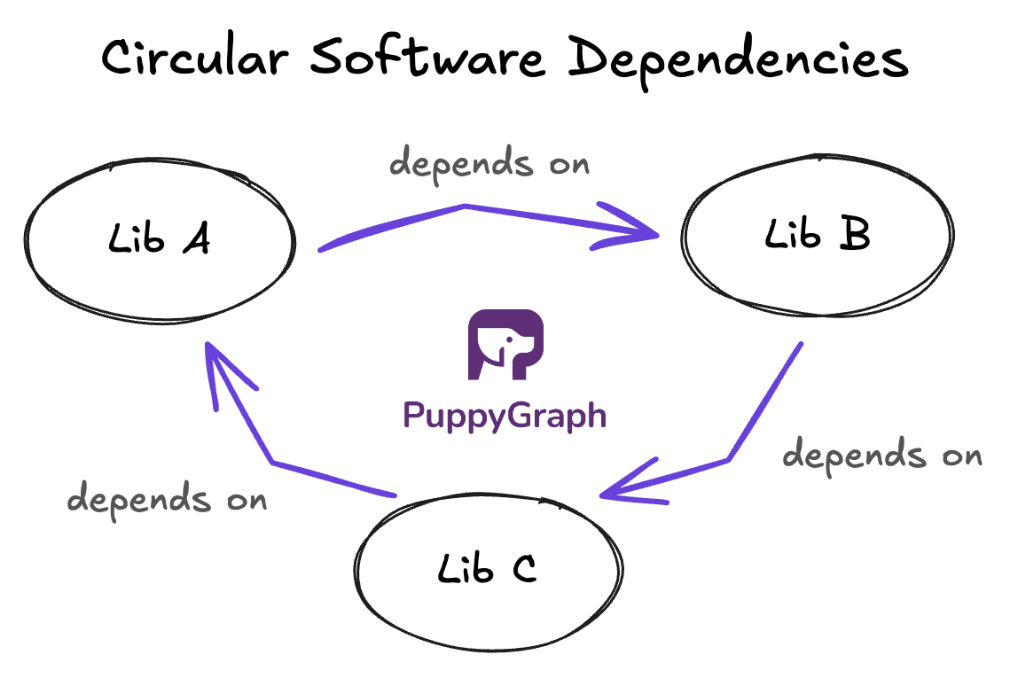
A cycle is a path that starts and ends at the same node, with no other node repeated. You follow edges from a node, visit a sequence of distinct nodes, and arrive back where you started.

Cycles tell you that there are feedback loops or circular dependencies in your structure:

• Software dependency graphs: a library A depends on B, B depends on C, and C depends (directly or indirectly) on A again, creating a dependency cycle.
• Fraud graphs: a group of accounts, devices, or merchants repeatedly transact with each other in a loop, forming a fraud ring where money circulates.
• Compliance graphs: roles or approvers are wired so that approvals eventually route back to the original approver, creating a circular approval that can block real sign off.

In directed graphs, you talk about directed cycles, where all edges in the cycle follow a consistent direction. 

Graphs with no directed cycles are called directed acyclic graphs (DAGs), which means you can follow the arrows, but you can never return to your starting point. DAGs are common in task scheduling and data pipelines because they encode flows that move forward without looping back.

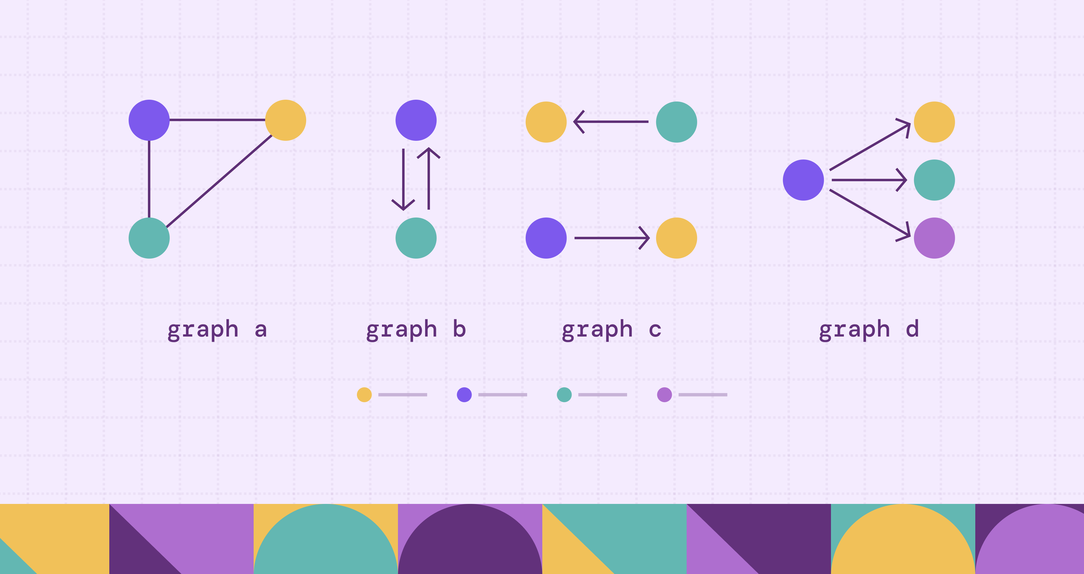
Types of Graphs Based on Nodes and Edges

Once you have nodes and edges, you can start to classify graphs based on how those edges behave and how they connect nodes. These types show up again and again in both theory and real datasets.

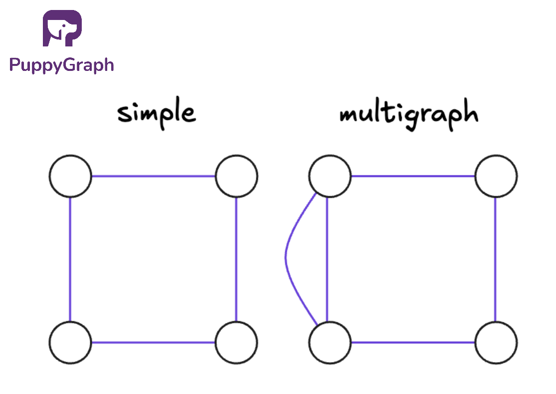
Simple and Multigraphs

A simple graph follows two basic rules:

• At most one edge between any pair of nodes
• No self loops

Either there is an edge between two nodes, or there is not.

A multigraph relaxes the rules of a simple graph. It allows multiple edges between the same pair of nodes, and often allows self loops as well. Multigraphs are handy when you want to capture repeated or parallel relationships, such as multiple transactions between the same two accounts or several distinct connections between the same pair of services.

Directed and Undirected

In an undirected graph, edges have no direction. The connection between u and v is the same as between v and u. Relationships like “friends with” or “shares subnet with” are usually modeled this way.

In a directed graph, each edge has a direction, from a source node to a target node. The edge (u,v) is different from (v,u). Relationships like “follows”, “child of”, or “can connect to” can be directional.

Weighted and Unweighted

In an unweighted graph, all edges are treated equally. For graph algorithms like shortest path and centrality, this means that we can take all edges as having a weight of 1. 

In a weighted graph, edges (and sometimes nodes) can carry numeric values, such as distance, latency, cost, or risk. Once weights are present, shortest paths and centrality start to depend on those values, not just the number of hops.

Labeled and Unlabeled

In an unlabeled graph, nodes are treated as anonymous. You only care about the shape of the graph, not which specific node is which. Two unlabeled graphs are considered the same if you can rename their nodes and get the same connections. This view is common in pure graph theory, where the focus is on structure, like “a triangle plus a tail,” not on identities.

In a labeled graph, nodes and edges have identifiers, names, or types attached. In practice, almost every real-world graph is labeled in some way. An example cybersecurity graph might look as follows:

Labels help you distinguish different kinds of entities and relationships. They let you ask targeted questions such as “paths from public subnets to databases” or “users who follow and transact with the same accounts,” instead of treating all nodes and edges as interchangeable.

Property Graphs

A property graph is a graph model where nodes and edges can both carry key value properties in addition to their IDs and labels. Nodes can now capture attributes such as country, account_type, or risk_score, while edges can store details like latency_ms, risk_level, or last_seen_at.

These properties enrich the kinds of graph analytics you can run. The structure tells you who is connected to whom. The properties bring in real-world meaning, so you can ask questions like:

• Paths from public subnets to databases where at least one edge is high risk
• Users within two hops of a high value account created in the last 30 days
• Services that sit on many low latency paths between two critical regions

By combining graph structure with modeled entities and attributes, property graphs let you move from “what is connected” to “what is connected, under which conditions, and how important those connections are.”

Directed vs Undirected Graphs Explained

In an undirected graph, edges have no direction. An edge between u and v means “u is connected to v” and “v is connected to u” in exactly the same way. Relationships such as “friends with”, “shares subnet with” often fit this model.

In a directed graph, each edge has a direction. An edge (u,v) goes from u to v. This lets you model asymmetric relationships, such as:

• “Service A calls Service B”
• “Role A can assume Role B”
• “Packet can flow from subnet A to subnet B”

Reachability now depends on edge direction. There might be a path from u to v, but not from v to u.

Expressing Undirected Graphs as Directed Graphs

Any undirected graph can be represented as a directed graph if you replace each undirected edge {u,v} with two directed edges:

\[\{u, v\} \quad \to \quad (u, v) \text{ and } (v, u)\]

The result is a directed graph where every connection is symmetric. 

Connected Components

Direction also affects how you think about connectivity.

For undirected graphs, a connected component is a maximal group of nodes where each node is reachable from every other node in that group. Maximal means that you cannot add any other nodes from the graph and still keep the subgraph connected.

For directed graphs, there are two common notions of components:

• Strongly connected components: every node is reachable from every other node by following edge directions.
• Weakly connected components: you ignore edge directions and then find connected components as if the graph were undirected.

Weakly connected components tell you how the graph clusters if you only care that a link exists, not which way it points. This is useful when you want to see the overall “island” structure of a directed graph, such as:

• Groups of services that are linked by any call in either direction
• Regions of an identity or permissions graph where any access relationship exists between nodes

Strong connectivity is stricter and direction aware. Weak connectivity ignores direction and focuses on whether nodes belong to the same piece of the graph at all.

Weighted and Unweighted Graphs: What’s the Difference?

So far, we have treated edges as either present or absent. That is an unweighted graph. 

In many real problems, though, not all connections are equal. Some are shorter, cheaper, faster, or riskier than others. That is where weights come in. In a weighted graph, edges (and sometimes nodes) carry numeric values. Formally, you can think of a weight function

\[w: E  \rightarrow \mathbb{R}\]

that assigns a number to each edge. That number can represent the cost of using a link or taking an action:

• Distance in a road network
• Latency or bandwidth between services
• Risk or likelihood in a security or fraud graph

Weights change both which graph algorithms you use and what their results mean. In unweighted graphs, shortest paths and centrality often treat every edge as having cost 1, so simple breadth first search is enough and “shortest” means fewest hops. 

In weighted graphs, you need weight aware algorithms like Dijkstra or Bellman–Ford, and “shortest” means minimum total weight. The same idea carries over to spanning trees (minimum spanning trees instead of any tree) and centrality and community detection, which can rank nodes and clusters based on low cost, low latency, or strong connections rather than just raw connectivity.

How Nodes and Edges Represent Real-World Data

At a high level, graphs let you turn “things and how they relate” into nodes and edges. A node stands for an entity in your system, and an edge stands for a relationship between two entities. The same raw data can be modeled in different ways, depending on what questions you care about.

You choose what a node represents based on your problem space and the level of detail you need. A node could be a user, device, IP address, services, and subnets. Edges then encode how those entities relate, such as “follows”, “owns”, “calls”, or “runs on”.

Real-world graphs usually use typed nodes and edges with attributes. In a property graph, for example, nodes have labels (User, Machine, Role, Product) and key value properties like country, risk_score, or created_at. Edges do the same with labels such as FOLLOWS, DEPENDS_ON, HAS_ACCESS_TO, plus properties like since, weight, or latency_ms. Structure gives you connectivity, while attributes give you the context you filter and rank on.

Some examples include:

• Cybersecurity Graphs
  
  • Nodes: VM Instances, Roles, Resources, Security Groups, Subnets
  • Edges: “assigned role”, “allows access to”, “contains”, “gateway to”

• Social Networks
  
  • Nodes: users, groups, posts, events
  • Edges: “follows”, “friend of”, “joined”, “liked”, “replied to”

• eCommerce Graphs
  
  • Nodes: Customers, Orders, Products, Suppliers
  • Edges: “viewed”, “added to cart”, “purchased”, “belongs to order”

The power of graphs comes from matching your domain to nodes, edges, and attributes in a way that mirrors how your system behaves. Once that mapping is in place, many questions about reachability, influence, risk, and similarity become graph queries on top of your data.

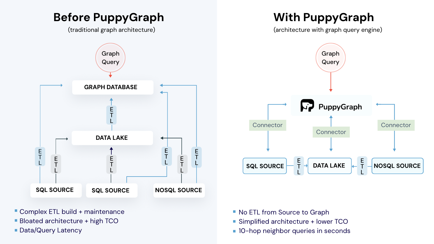
Challenges in Managing Large-Scale Node-Edge Graphs

In real production environments, enterprises and organizations generate large amounts of data that may be stored in many places, including data lakes, data warehouses, and databases. Large-scale node-edge graphs are modeled from this data and can then be used for graph analysis and graph queries. Traditional methods require building and maintaining a complex ETL system to load the data into a dedicated graph database. More specifically, this approach encounters several challenges:

• Integration and migration: Moving from relational tables to nodes and edges requires complex ETL and custom integrations, which are error prone and hard to keep in sync with existing systems.
• Data modeling and schema design: Flexible or schema-less models can drift over time, and evolving graph topologies make it difficult to design schemas that stay both clean and performant over time.
• Performance and scalability: Multi-hop traversals are hard to optimize and graphs are difficult to shard, so cross partition queries add latency and make large graph databases challenging to scale.

How PuppyGraph Helps

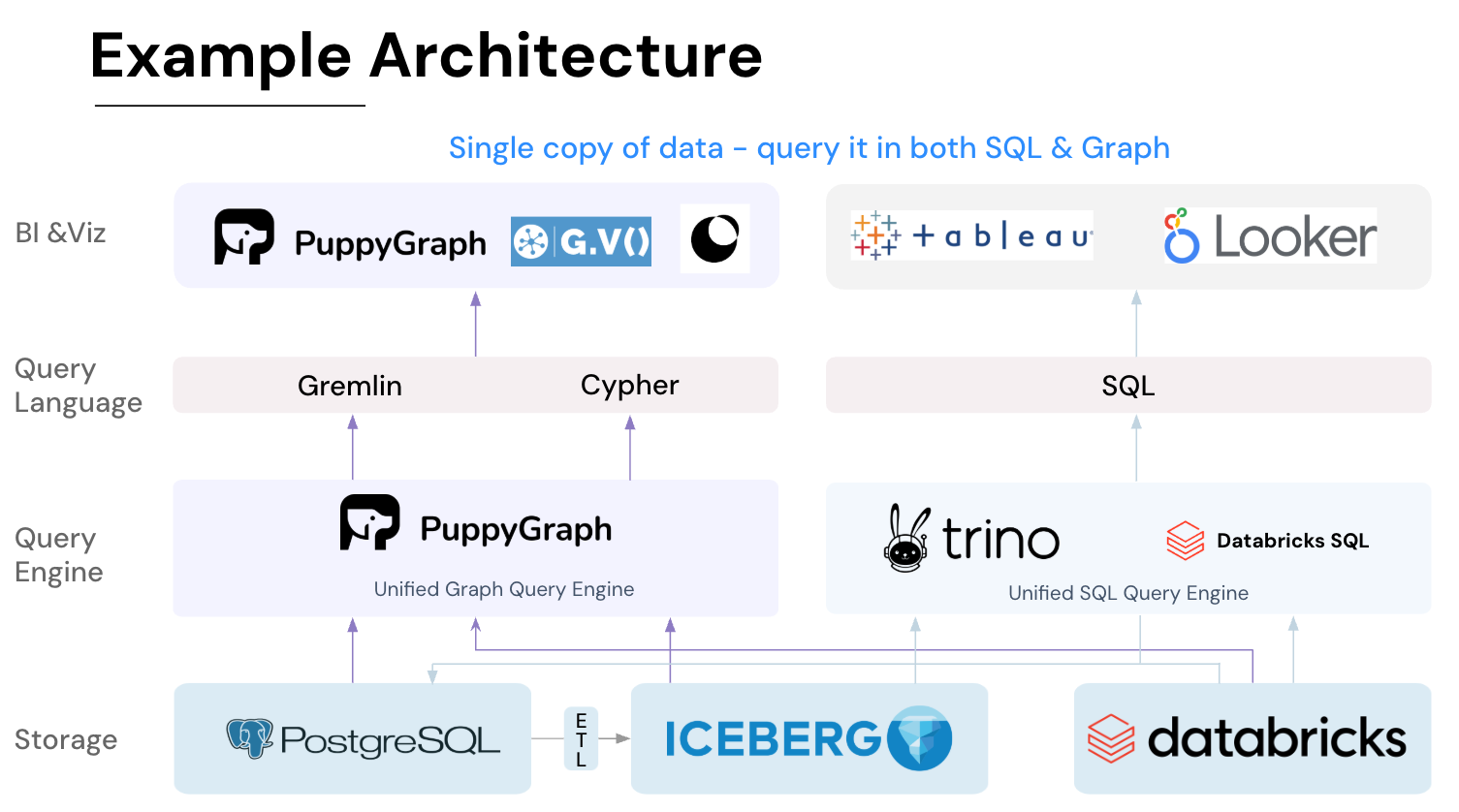
PuppyGraph is the first and only real time, zero-ETL graph query engine in the market, empowering data teams to query existing relational data stores as a unified graph model that can be deployed in under 10 minutes, bypassing traditional graph databases' cost, latency, and maintenance hurdles.

It seamlessly integrates with data lakes like Apache Iceberg, Apache Hudi, and Delta Lake, as well as databases including MySQL, PostgreSQL, and DuckDB, so you can query across multiple sources simultaneously.

Key PuppyGraph capabilities include:

• Zero ETL: PuppyGraph runs as a query engine on your existing relational databases and lakes. Skip pipeline builds, reduce fragility, and start querying as a graph in minutes.

• No Data Duplication: Query your data in place, eliminating the need to copy large datasets into a separate graph database. This ensures data consistency and leverages existing data access controls.

• Real Time Analysis: By querying live source data, analyses reflect the current state of the environment, mitigating the problem of relying on static, potentially outdated graph snapshots. PuppyGraph users report 6-hop queries across billions of edges in less than 3 seconds.

• Scalable Performance: PuppyGraph’s distributed compute engine scales with your cluster size. Run petabyte-scale workloads and deep traversals like 10-hop neighbors, and get answers back in seconds. This exceptional query performance is achieved through the use of parallel processing and vectorized evaluation technology. 

• Best of SQL and Graph: Because PuppyGraph queries your data in place, teams can use their existing SQL engines for tabular workloads and PuppyGraph for relationship-heavy analysis, all on the same source tables. No need to force every use case through a graph database or retrain teams on a new query language.

• Lower Total Cost of Ownership: Graph databases make you pay twice — once for pipelines, duplicated storage, and parallel governance, and again for the high-memory hardware needed to make them fast. PuppyGraph removes both costs by querying your lake directly with zero ETL and no second system to maintain. No massive RAM bills, no duplicated ACLs, and no extra infrastructure to secure.

• Flexible and Iterative Modeling: Using metadata driven schemas allows creating multiple graph views from the same underlying data. Models can be iterated upon quickly without rebuilding data pipelines, supporting agile analysis workflows.

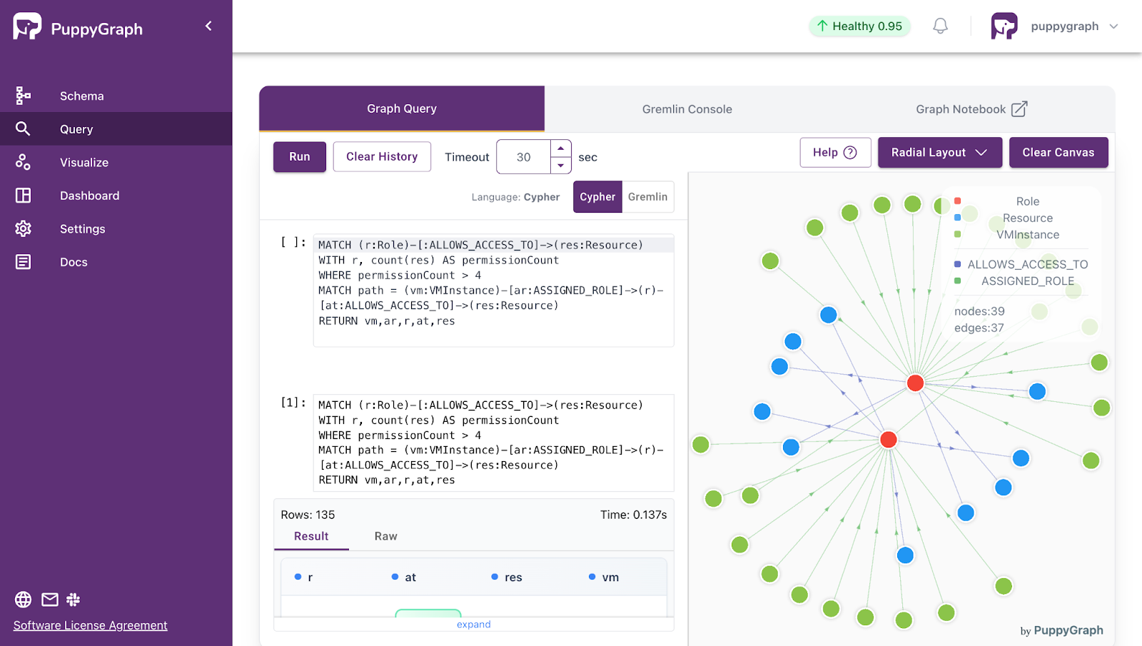
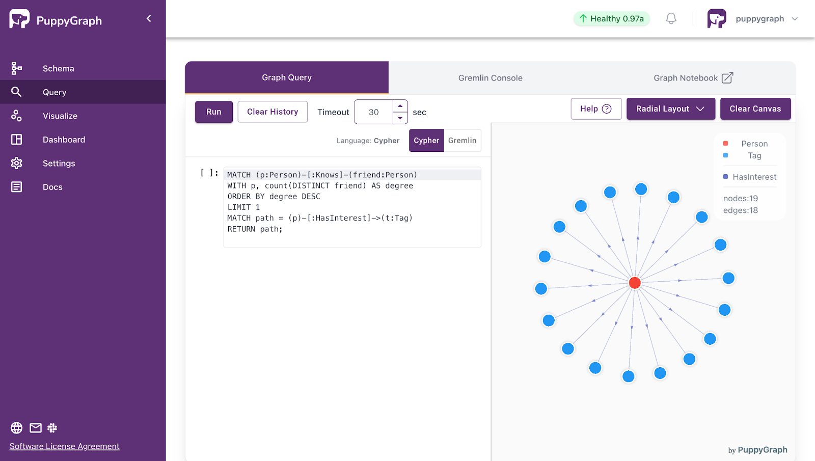
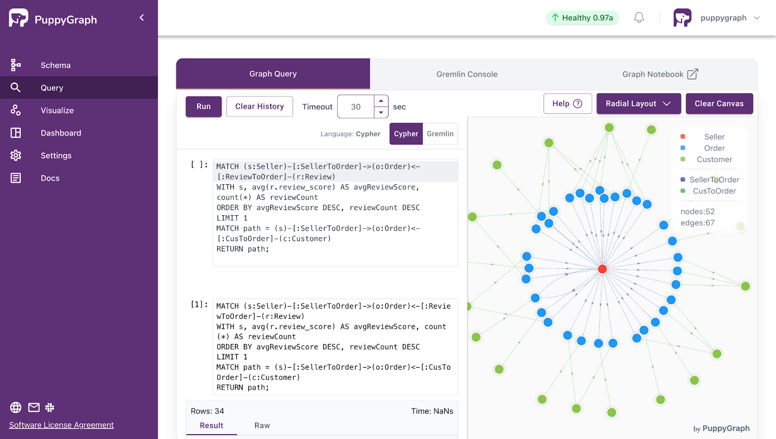
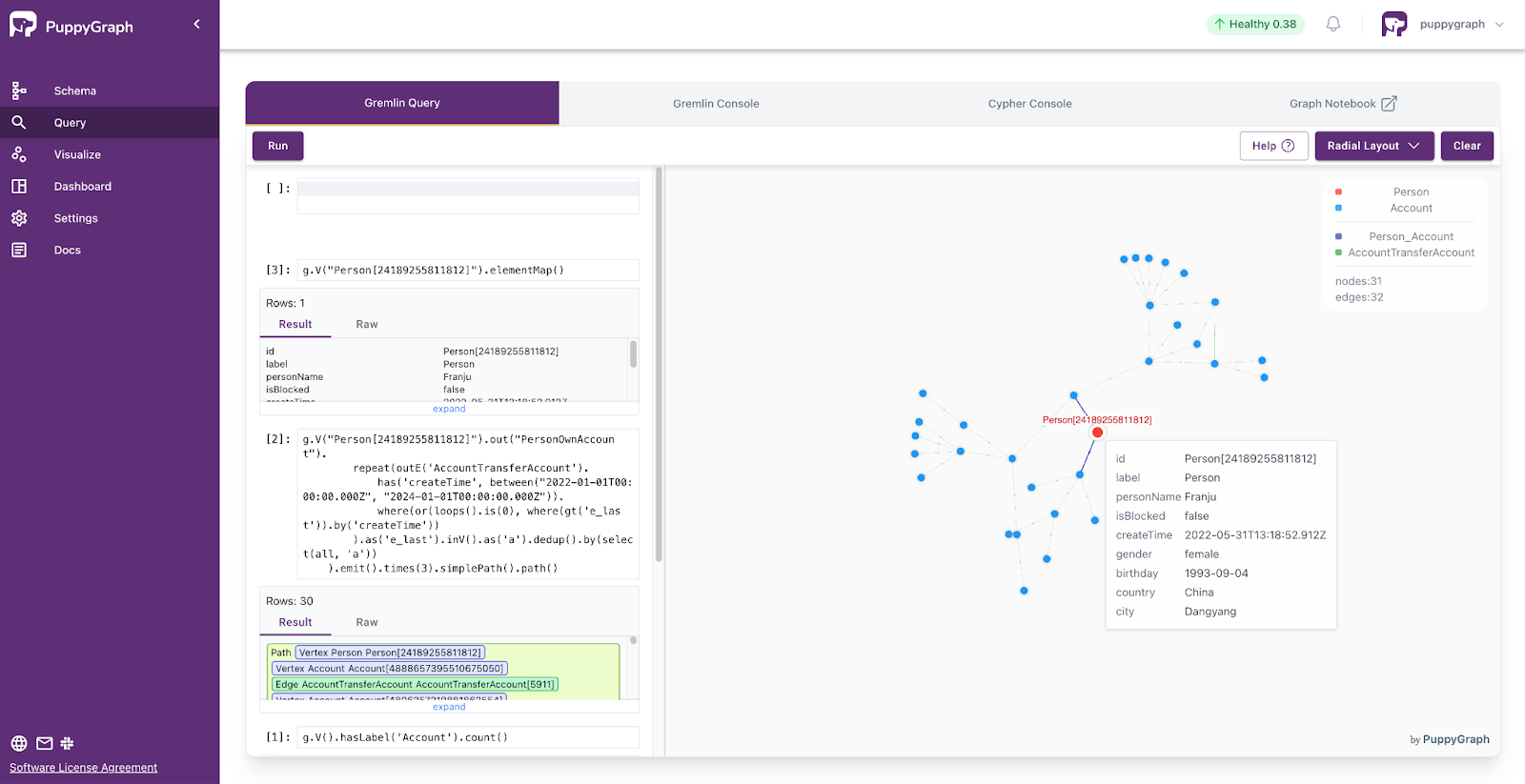
• Standard Querying and Visualization: Support for standard graph query languages (openCypher, Gremlin) and integrated visualization tools helps analysts explore relationships intuitively and effectively.

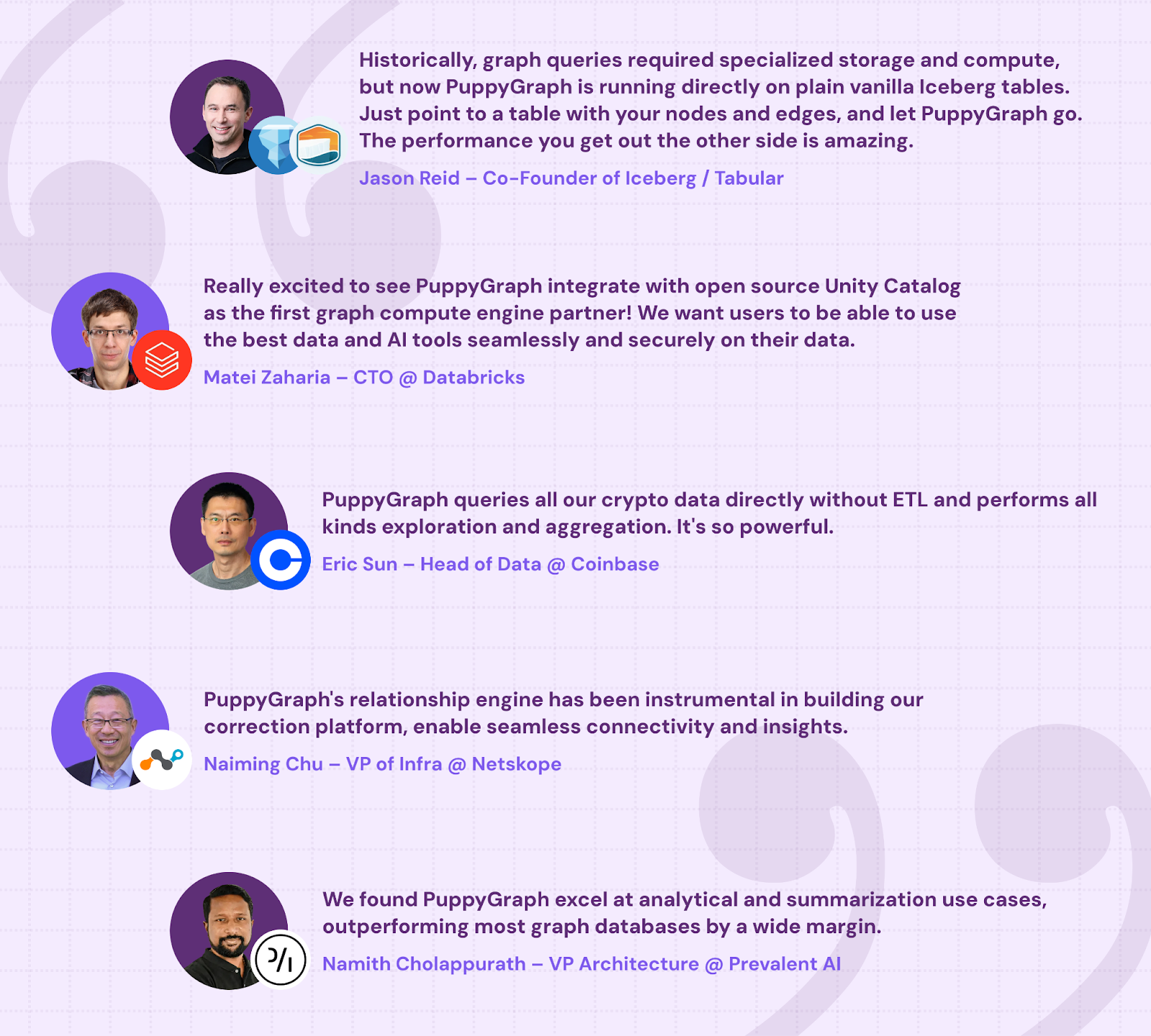
• Proven at Enterprise Scale: PuppyGraph is already used by half of the top 20 cybersecurity companies, as well as engineering-driven enterprises like AMD and Coinbase. Whether it’s multi-hop security reasoning, asset intelligence, or deep relationship queries across massive datasets, these teams trust PuppyGraph to replace slow ETL pipelines and complex graph stacks with a simpler, faster architecture.

As data grows more complex, the most valuable insights often lie in how entities relate. PuppyGraph brings those insights to the surface, whether you’re modeling organizational networks, social introductions, fraud and cybersecurity graphs, or GraphRAG pipelines that trace knowledge provenance.

Deployment is simple: download the free Docker image, connect PuppyGraph to your existing data stores, define graph schemas, and start querying. PuppyGraph can be deployed via Docker, AWS AMI, GCP Marketplace, or within a VPC or data center for full data control.

Conclusion

Graphs give you a clean way to think about complex systems. By modeling your world as nodes and edges, you can see surface structures that hide within your data: how identities gain access, how services call each other, how customers move through products, and where cycles, weak points, or clusters appear. Once your data is in a graph shape, questions about reachability, influence, and risk become graph queries instead of guesswork.

Want to bring graph thinking straight to where your data lives? Download PuppyGraph’s  forever-free Developer Edition or book a demo with the PuppyGraph team to walk through your use case from modeling nodes and edges to running multi hop queries over real workloads.