

Many-to-Many Relationship: Explained
Many-to-many relationships sound simple at first. Picture a school roster. Many students can enroll in a class, and each student can take multiple classes. Many students to many classes. The idea seems fairly intuitive.
In practice, it gets a lot trickier. Do you also model instructors who teach many classes and interact with many students? Which of those links matter for your use case right now? Will they matter in future? Those choices shape your schema and how it performs as the dataset grows. Imagine the complexity in massive real-world datasets with millions of records and highly connected entities.
These relationships show up because real systems are shared and reusable. People join groups, items sit in multiple buckets, and actions connect to more than one thing. You will run into them anytime both sides of a relationship can link to several items on the other side.
This blog walks through what many-to-many relationships mean in databases, how they are modeled, and what to consider as data grows. We will cover the core structure, a concrete SQL example, and the tradeoffs around indexing, constraints, and reporting so you can keep your model clear and performant.
What is a Many-to-Many Relationship?
Relational models define relationships between tables, including cardinality, which describes how many records on one side can link to how many on the other. When creating Entity Relationship (ER) diagrams using Crow’s foot notation, we note three types of cardinality:
- One-to-One (1:1): One record in A connects to one record in B. Example: Each student has one student ID card, and each ID card belongs to one student.
- One-to-Many (1:N): One record in A connects to many records in B. Example: Each class consists of multiple students.
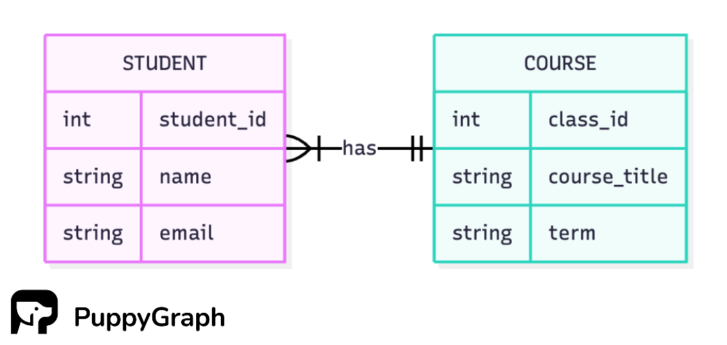
- Many-to-Many (N:M): Many records in A connect to many records in B. Example: Each student can take multiple classes and each class can include multiple students.
You’ll notice we use the student–course pair to illustrate both one-to-many and many-to-many. That’s because cardinality follows your business rules. If every student has a single primary class, it’s one-to-many. If students can take multiple classes and classes include multiple students, it’s many-to-many and you need an enrollment table.

Here are some quick checks you can do to tell if your tables hide a many-to-many relationship:
- Ask the quick questions: Can one A link to multiple B? Can one B link to multiple A? If both are true, you likely have a many-to-many relationship.
- Scan for repeats: Do keys on both sides appear more than once in the link (or prospective link) data? Repeats on both sides indicate a many-to-many relationship.
- Spot modeling smells: Comma-separated ID lists, owner_id_1/owner_id_2/... columns, or frequent duplicated rows to represent links.
- Look for relationship attributes: Do you need fields that belong to the link itself (e.g., role, quantity, price-at-time, effective dates)? That points to a junction table.
- Check query needs: Do you regularly ask in both directions (“who follows me” and “who do I follow”) or chain multiple hops? That’s classic N:M usage.
- Consider time scope: Within a short window it might look 1:N, but across history it may be N:M. If time matters, evaluate within the right window.
Real-World Examples of Many-to-Many Relationships
Many-to-many relationships do more than link records. They carry meaning. They show up everywhere because the same thing often belongs to several contexts at once, and modeling these relationships provides insight that can drive high-impact decisions.
Cybersecurity
- Identities ↔ Groups/Roles (MEMBER_OF): A user can join many groups, and each group has many users.
- Users ↔ Resources via policies (CAN_ACCESS): Many users can reach a resource, and each user reaches many resources.
- Assets ↔ Vulnerabilities (HAS_VULN): A CVE affects many assets, and assets can have many CVEs.
Supply Chain
- Products ↔ Components (HAS_COMPONENT): A product consists of many components, and a component can appear in many products.
- Products ↔ Suppliers (SUPPLIED_BY): A product has multiple suppliers, and a supplier serves many products.
- Shipments ↔ Orders (FULFILLS): A shipment can cover many orders, and an order can be split across many shipments.
Finance
- Customers ↔ Accounts (OWNS): A customer can open many accounts, and an account can have multiple owners (joint accounts).
- Cards/Wallets ↔ Merchants (PURCHASED_AT): A card pays many merchants, and a merchant receives many cards.
- Accounts ↔ Devices (USES): An account can be accessed from many devices, and a device can be used by many accounts.
Social Networks
- Users ↔ Users (Follows) (FOLLOWS, FOLLOWED_BY): A user follows many users, and is followed by many users.
- Users ↔ Posts (REACTED_TO): A user reacts to many posts, and posts receive reactions from many users.
- Posts ↔ Hashtags (TAGGED_WITH): A post includes many tags, and a tag appears on many posts.
Healthcare
- Patients ↔ Providers (TREATED_BY): A patient sees many providers, and providers treat many patients.
- Patients ↔ Diagnoses/Conditions (HAS_DIAGNOSIS): A patient can have many conditions, and a condition is recorded across many patients.
- Patients ↔ Medications (PRESCRIBED): A patient takes many kinds of medication, and each medication can be prescribed to many patients.
How Many-to-Many Relationships Work in Databases
We often picture many-to-many relationships in simple terms: Users follow users, customers own accounts, products appear on orders. Databases don’t store them that way. Let’s walk through a few examples to see how the logical view differs from the physical model.
Example 1: Social Networks
At the concept level, users follow users. Both ends are the same entity, and the link is directional. That is the logical model: a user can follow many other users and can be followed by many users.
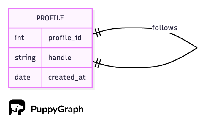
The idea is clear, but how should we store it? Putting follower data on the profile table breaks down. You would either cram a list of user IDs into one column or duplicate profile rows. A cleaner approach is a join table that records each follower–followee pair.
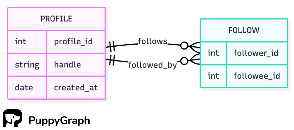
Since both foreign keys in the junction table point to the same primary key in the profile table, this is also known as a self-referential relationship. When you query it, you use self-joins so the profile table can play both roles.
Example 2: Financial Services
A customer can hold many accounts, and an account can have multiple owners.

Many-to-many relationships don’t have to use join tables, but it’s usually the better choice in relational databases. Before we jump into the “good” model, it helps to see the “bad” one:
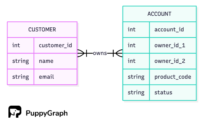
Storing all owners on the account row creates a multitude of problems. Most accounts aren’t joint, so a column like owner_id_2 sits empty and wastes space. It also hardcodes a limit; if you ever need three owners, you’re changing the schema. To keep concerns separate, we add a join table that records each customer–account relationship.

Example 3: eCommerce
An order can contain many products, and a product can appear in multiple orders.
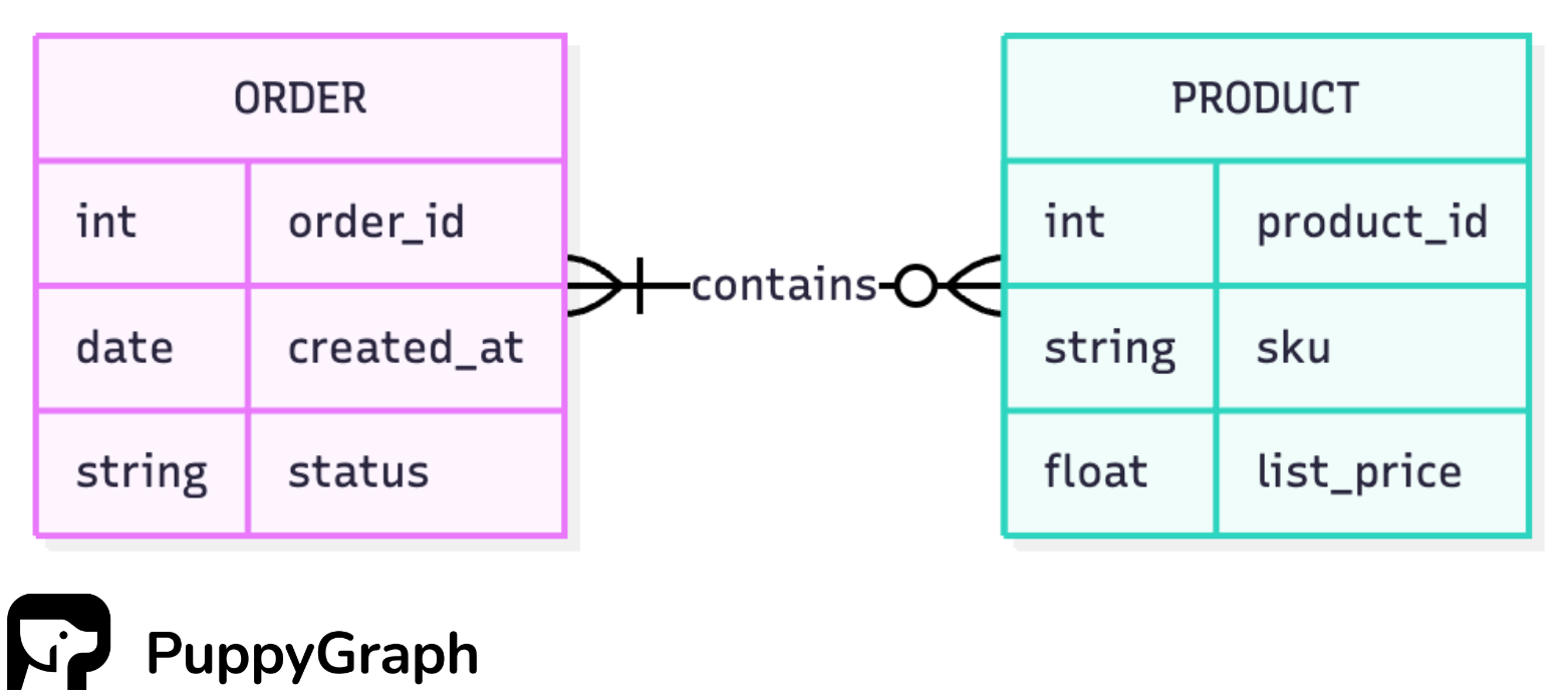
Join tables let you describe the relationship, not just connect two rows. These fields belong to the link and are usually unique to it. In Product ↔ Order, the order line stores quantity, the price charged at the time, and timestamps. Putting those on PRODUCT or ORDER would be awkward. Keeping them on the join keeps the meaning and history in the right place.

Advantages of Many-to-Many Relationships
When tackling many-to-many relationships, the benefits depend on how you execute the model. In practice, you’ll choose between a normalized approach and a denormalized one.
Normalized
Normalizing your many-to-many relationships means introducing a junction table that splits one N:M link into two 1:N links.
When you model many-to-many with a junction table, you express important relationships in a form that’s both accurate and efficient. Each link is one row instead of bloated arrays, duplicate columns, or NULL-heavy placeholders. Core tables stay narrow and focused on their own attributes, which can lead to better cache locality and less wasted memory. Foreign keys and a composite key keep pairs valid and unique, so updates touch a single place and your data stays clean.
Normalizing your many-to-many relationships lets you keep entities focused on what they are, and put facts about their connection in the junction. Customers keep profile data, products keep catalog data, and the order line holds quantity and price at purchase time. This split avoids stuffing relationship fields into parent tables, reduces NULL-heavy columns, and lets each side evolve independently. It also makes operations simple: adding or removing a link is a single insert or delete in one place, and you can enforce clear rules right where the relationship lives.
Queries stay intuitive when the junction table makes the connections explicit: one row equals one link. You filter the junction first, then join to the entities you need, which mirrors how you think about the question: who follows me, which products are on this order, which accounts a customer owns. The schema matches the mental model, so queries remain simple and correct as the system grows.
Junction tables cut redundancy, which cuts storage. Instead of repeating the same customer or product attributes across many rows, you store each entity once and keep just the pair in the junction. As fan-out grows, that difference adds up: base tables stay small, indexes stay leaner, and updates touch a single row instead of many copies. The result is less disk space, fewer write amplification issues, and a schema that scales without duplicating data just to represent links.
Denormalized
Denormalizing a many-to-many relationship means duplicating data so each table (or document) has the pieces it needs for the target queries. Instead of a single junction table, you might keep lists of related IDs, small embedded documents, or prejoined tables tailored to how the app reads.
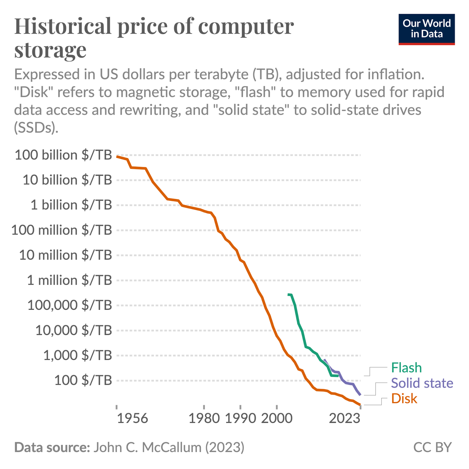
The main reason teams keep denormalized many-to-many relationships is speed. By duplicating data, you avoid joins on a junction table and can fetch exactly what you need with a single lookup. That keeps latency low and throughput high when reads dominate. As storage costs continue to reach historical lows, it can be a sensible trade-off to make when your product demands fast, predictable queries.
NoSQL databases tend to benefit more from many-to-many relationships because they aren’t constrained by SQL’s rigid joins and foreign-key rules. Document stores can embed related IDs or subdocuments right where reads happen, turning common queries into single-key lookups. Wide-row systems like Cassandra lean into denormalization and let you model “tables per access pattern” (e.g., followers_by_user, following_by_user) for predictable, fast reads at scale. Graph databases go further by making relationships first-class edges, so N:M links are natural and traversals don’t require joins.
Many-to-Many Relationship Example in SQL
Normalizing the many-to-many relationships is often the way to go when it comes to SQL databases. We’ll use the follower–followee pattern because it’s the simplest way to see how to model the link.
- Profile Table
CREATE TABLE profile (
    profile_id INT PRIMARY KEY,
    handle VARCHAR(50) NOT NULL,
    created_at TIMESTAMP DEFAULT CURRENT_TIMESTAMP
);- Follow Table
CREATE TABLE follow (
  follower_id INT NOT NULL,
  followee_id INT NOT NULL,
  PRIMARY KEY (follower_id, followee_id),
  FOREIGN KEY (follower_id) REFERENCES profile(profile_id) ON DELETE CASCADE,
  FOREIGN KEY (followee_id) REFERENCES profile(profile_id) ON DELETE CASCADE
);
The follow table uses a composite primary key on (follower_id, followee_id) to enforce uniqueness so you don’t end up with duplicate links. Both columns are foreign keys back to profile(id), which keeps referential integrity tight and makes updates and deletes straightforward: remove the row to unfollow, insert the row to follow, and let the database handle the rest.
We can then run an example query to see who follows a given user with user id 123:
SELECT p.*
FROM follow f
JOIN profile p ON p.profile_id = f.follower_id
WHERE f.followee_id = 123;
Challenges and Considerations
Data Integrity
Many-to-many links are easy to get wrong without guardrails. Prevent duplicate pairs with a composite primary key on the junction (e.g., (a_id, b_id)), block orphan links with foreign keys, and add checks for business rules like “no self-follows” or valid date ranges. If you denormalize, you lose DB-enforced integrity. You can compensate with idempotent writes, uniqueness guards, and periodic consistency checks.
Query Performance
Joins are cheap in small doses and brutal at scale. Many-to-many queries can explode row counts, and multi-hop paths turn into wide, memory-hungry joins. When questions routinely span three or more hops, a graph approach helps. Graph engines evaluate traversals without stitching huge join results, so path-heavy queries run faster and stay simpler to write.
Indexing Strategy
Start with two essentials: the composite primary key (a_id, b_id) and a reverse lookup index (b_id, a_id). Then add selective composites that match real filters (e.g., (followee_id, follower_id), (account_id, role), (order_id, product_id), (product_id, added_at)). Keeping indexes lean is still important since every extra index slows writes. For heavy writes, consider partial indexes or covering indexes tuned to your most frequent queries.
Schema Drift
Logical ER diagrams show a clean N:M, but production schemas grow fields for history, status, and operational flags. Keep a “physical model” alongside the logical diagram and document ownership of relationship fields. Review constraints and indexes as columns are added. Otherwise, you might end up with unused indexes, inconsistent nullability, and relationships that don’t match the diagram anymore.
Modeling Scope and Time
Cardinality depends on scope. Per term a student might have one homeroom (1:N), across years it’s N:M. Make the time basis explicit: add effective_from/effective_to on the junction, filter for “active” links in current views, and keep history for audits and point-in-time reports. Define whether timestamps come from the entity or the relationship, and stick to that grain to avoid double counting.
How PuppyGraph Can Help
Relational databases aren’t relationship-first. Many-to-many links sit behind joins, so the moment you ask path-heavy questions, queries fan out and slow down. If your goal is to understand how entities relate to one another across several hops, you end up relying on brittle table joins that quickly become hard to read.
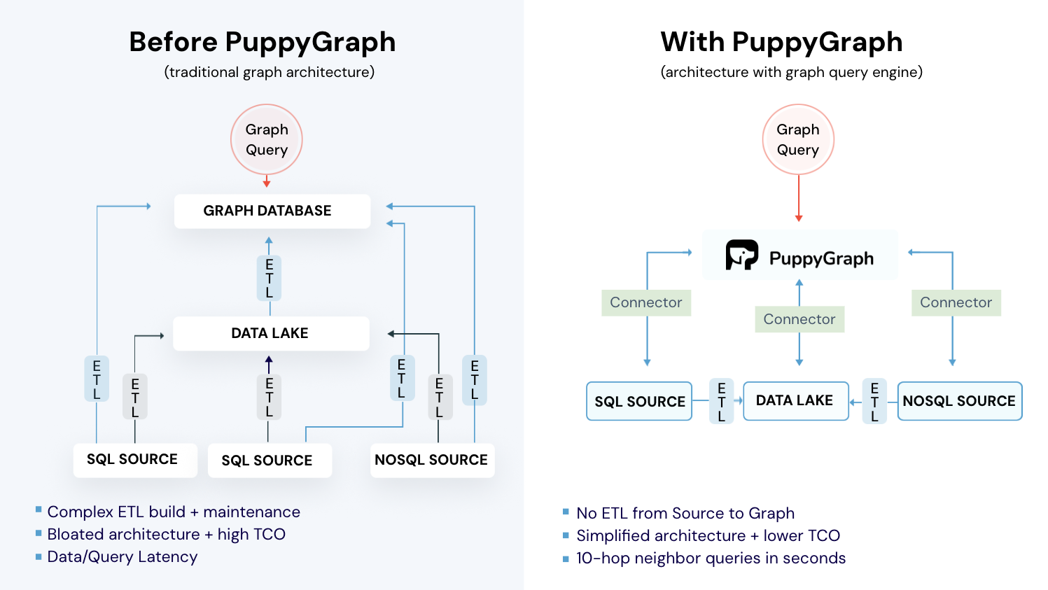
Graph databases solve the traversal problem, but they usually require a separate store. That means ETL, duplicated data, lag between systems, and more infrastructure to run and secure. For many teams, the cost outweighs the benefit.
PuppyGraph takes a different route. It plugs graph query analytics directly into your existing relational databases. You keep your schema, your tables, and your SQL.

Instead of migrating data into a specialized store, PuppyGraph connects to sources including PostgreSQL, Apache Iceberg, Delta Lake, BigQuery, and others, then builds a virtual graph layer over them. Graph models are defined through simple JSON schema files, making it easy to update, version, or switch graph views without touching the underlying data.Key PuppyGraph capabilities include:
- Zero ETL: PuppyGraph runs as a query engine on your existing relational databases and lakes. Skip pipeline builds, reduce fragility, and start querying as a graph in minutes.
- No Data Duplication: Query your data in place, eliminating the need to copy large datasets into a separate graph database. This ensures data consistency and leverages existing data access controls.
- Real Time Analysis: By querying live source data, analyses reflect the current state of the environment, mitigating the problem of relying on static, potentially outdated graph snapshots. PuppyGraph users report 6-hop queries across billions of edges in less than 3 seconds.
- Scalable Performance: PuppyGraph’s distributed compute engine scales with your cluster size. Run petabyte-scale workloads and deep traversals like 10-hop neighbors, and get answers back in seconds. This exceptional query performance is achieved through the use of parallel processing and vectorized evaluation technology.
- Best of SQL and Graph: Because PuppyGraph queries your data in place, teams can use their existing SQL engines for tabular workloads and PuppyGraph for relationship-heavy analysis, all on the same source tables. No need to force every use case through a graph database or retrain teams on a new query language.
- Lower Total Cost of Ownership: Graph databases make you pay twice — once for pipelines, duplicated storage, and parallel governance, and again for the high-memory hardware needed to make them fast. PuppyGraph removes both costs by querying your lake directly with zero ETL and no second system to maintain. No massive RAM bills, no duplicated ACLs, and no extra infrastructure to secure.
- Flexible and Iterative Modeling: Using metadata driven schemas allows creating multiple graph views from the same underlying data. Models can be iterated upon quickly without rebuilding data pipelines, supporting agile analysis workflows.
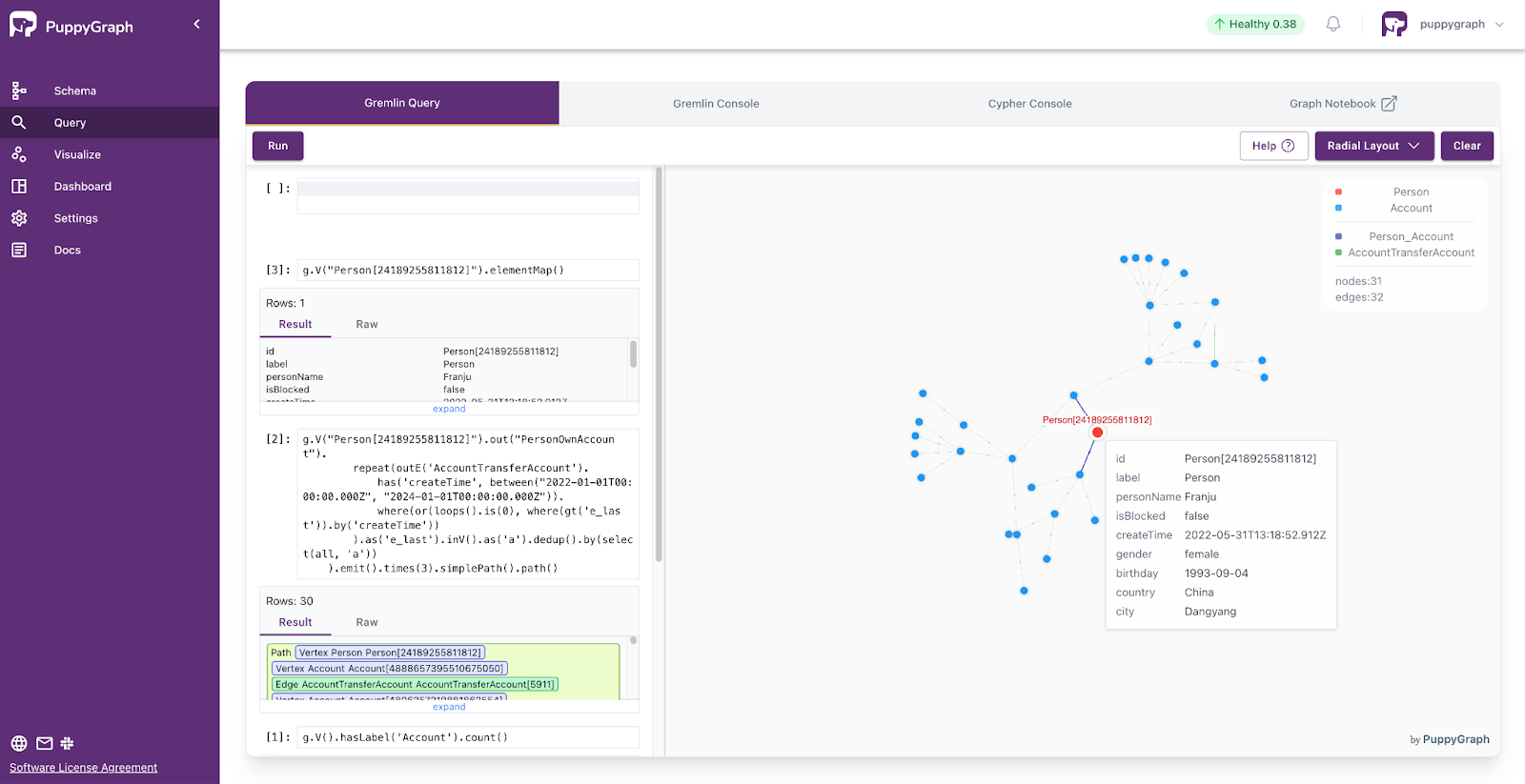
- Standard Querying and Visualization: Support for standard graph query languages (openCypher, Gremlin) and integrated visualization tools helps analysts explore relationships intuitively and effectively.
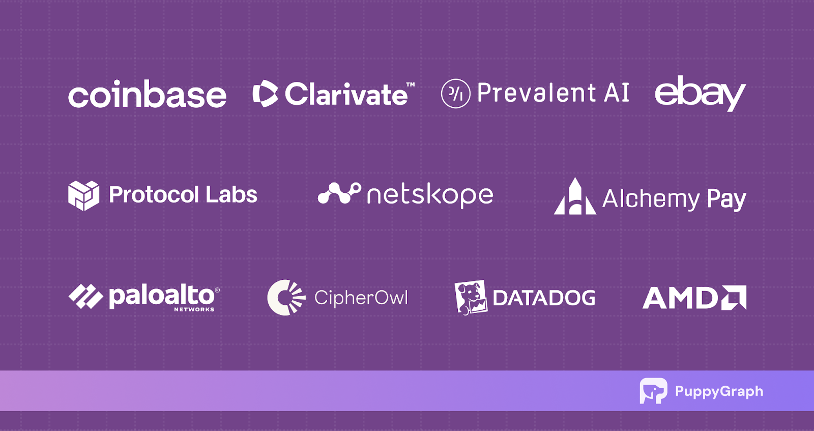
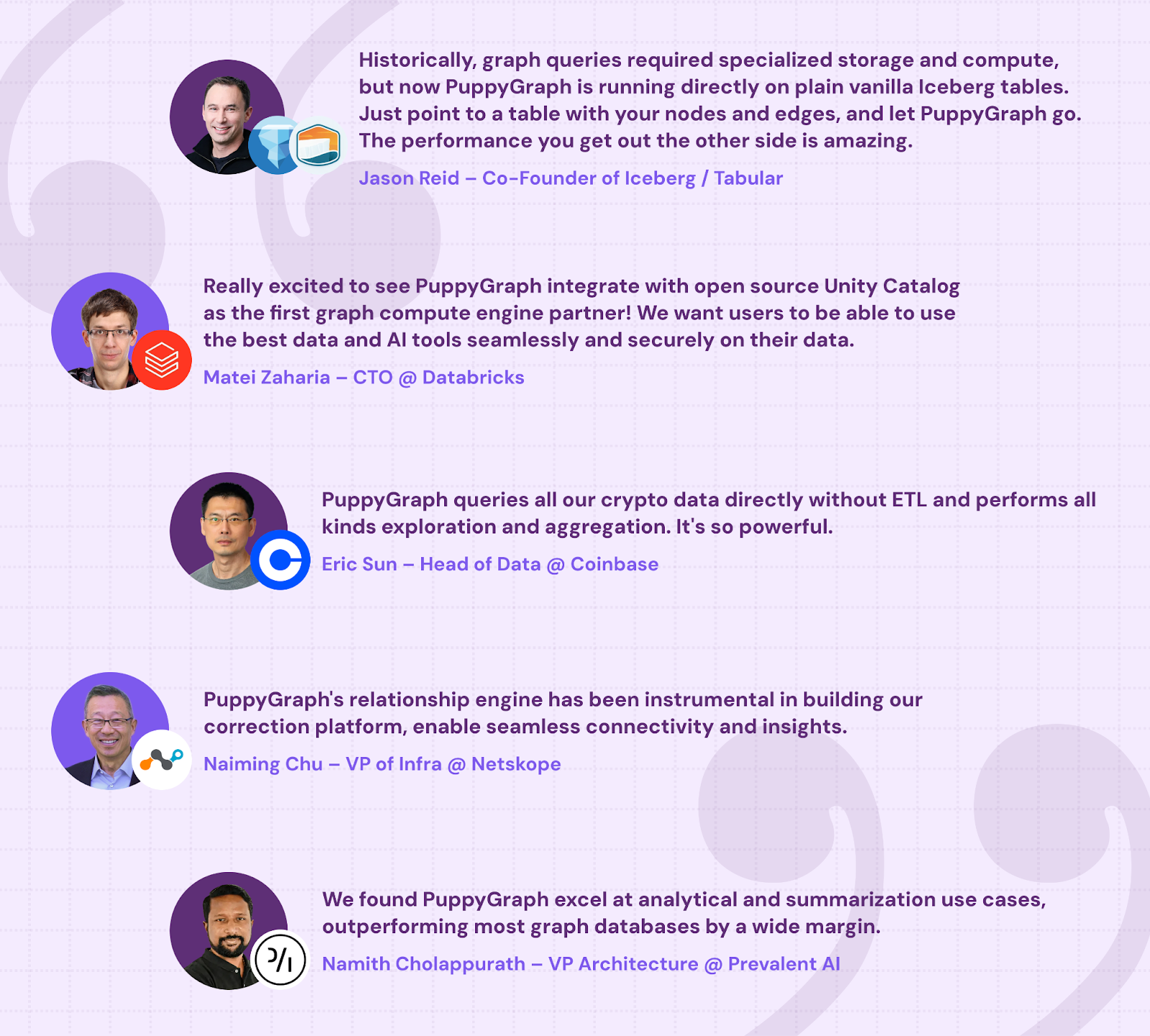
- Proven at Enterprise Scale: PuppyGraph is already used by half of the top 20 cybersecurity companies, as well as engineering-driven enterprises like AMD and Coinbase. Whether it’s multi-hop security reasoning, asset intelligence, or deep relationship queries across massive datasets, these teams trust PuppyGraph to replace slow ETL pipelines and complex graph stacks with a simpler, faster architecture.
As data grows more complex, the most valuable insights often lie in how entities relate. PuppyGraph brings those insights to the surface, whether you’re modeling organizational networks, social introductions, fraud and cybersecurity graphs, or GraphRAG pipelines that trace knowledge provenance.
Deployment is simple: download the free Docker image, connect PuppyGraph to your existing data stores, define graph schemas, and start querying. PuppyGraph can be deployed via Docker, AWS AMI, GCP Marketplace, or within a VPC or data center for full data control.
Conclusion
Many-to-many relationships are everywhere, and modeling them well is how you keep data accurate and useful. In SQL, junction tables shine for one- to two-hop questions and give you clean constraints, lean storage, and predictable queries. When you need deeper traversals or connection-heavy analytics, those joins start to drag.
That’s where PuppyGraph comes in. PuppyGraph is the first real-time, zero-ETL graph query engine, letting you run graph analytics directly on your existing SQL databases without compromising on speed. You keep your schema and data where they are, then use graph queries to traverse multiple hops quickly. Graph models are defined through simple JSON schema files, making it easy to update, version, or switch graph views without touching the underlying data. PuppyGraph provides a practical way to get path-heavy answers without a migration or a parallel data stack.
If you want to see what multi-hop queries feel like on your data, try our forever-free Developer edition, or book a demo with our team to get started.

Jaz Ku is a Solution Architect with a background in Computer Science and an interest in technical writing. She earned her Bachelor's degree from the University of San Francisco, where she did research involving Rust’s compiler infrastructure. Jaz enjoys the challenge of explaining complex ideas in a clear and straightforward way.

Get started with PuppyGraph!


Developer Edition
- Forever free
- Single noded
- Designed for proving your ideas
- Available via Docker install
Enterprise Edition
- 30-day free trial with full features
- Everything in developer edition & enterprise features
- Designed for production
- Available via AWS AMI & Docker install