Two simple numbers, node count and edge count, tell you a lot about how a graph will behave. They show size and composition, how connected the data is, and areas of interest within your data. Read together, they’re early signals for performance, scalability, and data quality.

In this blog, you’ll learn what node count and edge count reveal about your data and why they’re so useful for analytics. We’ll tie those numbers to real outcomes: where they help, where they hurt and how they influence query cost as graphs grow. We’ll finish with practical ways to get accurate counts in your own system so you can read these metrics with confidence.

What is Node Count?

Node count is the total number of distinct entities stored as nodes in your graph. Nodes are also called vertices, which is why node count is often written as V. Each node stands for something you care about, such as a user, device, order, repository, or IP.

Key Features

Node count is your quick read on how much “stuff” lives in the graph and how it’s spread across types. Important statistics that node counts can reveal include:

• Overall Data Volume: The total number of nodes shows the size of the graph and the number of distinct entities represented. 
• Distribution of Entity Types: Counting nodes by label or type (for example, “Person,” “Product,” “Location”) highlights which categories are most prevalent. This helps with profiling and understanding the graph’s composition.
• Potential for Bottlenecks or Areas of Interest: A high count for a particular type can point to central entities or highly connected regions worth analyzing or optimizing. A low count can flag rare entities or sparse areas.
• Data Quality and Completeness: Unexpected counts for certain types can signal duplicates, missing uniqueness constraints, or incomplete ingestion. 
• Impact of Data Changes: Tracking counts over time shows growth or shrinkage across types and helps you see how updates affect the dataset.

What is Edge Count?

Edge count is the total number of relationships in your graph, written as E. Each edge links two nodes to express something like follows, purchased, or connected_to. In most graph databases, edges are stored as directed, but you can query them either with direction or without direction, so the same relationship can be treated as directed when order matters and as undirected when it does not.

Key Features

Edge counts tell you how relationships are spread through the graph and where activity concentrates. Important statistics that edge counts can reveal include:

• Overall relationship volume: The total number of edges shows how much connectivity your graph carries.
• Distribution of relationship types: Counting edges by type highlights which interactions dominate and how the graph is composed.
• Connectivity hot spots: High edge counts around certain nodes or segments point to hubs, dense regions, or areas to optimize.
• Data quality and consistency: Unexpected spikes, duplicate links, or self-loops can signal ingestion or modeling issues.
• Change over time: Tracking edge counts by window reveals bursts, seasonality, and how relationships evolve.

What Count As Nodes vs Edges: Key Differences

Deciding what to model as a node versus an edge depends on your context, domain, and query patterns. If the graph model is not properly defined, it could paint a misleading picture about the data that you have. 

For example, determining whether a flight between airports should be considered a node or an edge can be tricky.

• As an edge: For route maps and simple schedules.

(:Airport)-[:FLIGHT {dep, arr}]->(:Airport) 

• As a node: For when you handle equipment, crew, seats, fares, delays, and connections to bookings.

(:Flight) 

Let’s take a look at some considerations to think about when determining what is a node and what is an edge.

Fundamental Roles

Nodes (vertices) represent the things in your domain. Edges represent the ties between those things. Model as a node when the item is a first-class entity you look up or secure. Model as an edge when you are describing how two existing nodes relate.

Information Conveyed

Both nodes and edges can contain properties, but they hold different kinds of properties. Nodes carry attributes about the entity itself, such as name, type, and status. Edges carry attributes about the relationship, such as timestamp, weight, role, or validity window.

Independence

A node has meaning on its own and can exist without any relationships. An edge depends on two valid endpoints and has no standalone meaning without them.

Multiplicity and Richness

When a relationship needs its own history, approvals, or many fields, consider promoting it to an intermediate node that sits between two entities. Ask: “Do I need to attach other relationships to this edge?” or “Do I need to version or permission this edge separately?” If yes, use a small node for the relationship instance.

Ratio of Nodes to Edges

Before we dive into the calculations, it can be helpful to understand the limits of how many nodes and edges a graph can have. 

For nodes, while there are no theoretical constraints, you're mostly limited by storage and governance. On the other hand, edges grow with connectivity and are bounded by V. Let’s take a look at the upper bounds for the number of edges various graph types can have:

• Simple, Undirected Graphs: \(|E|_{max}=\frac{|V|(|V|-1)}{2}\)
• Simple, Directed Graphs: \(|E|_{max}=|V|(|V|-1)\)

• Directed Graphs with Self-Loops: \(|E|_{max}=|V|^2\)

Checking bounds gives you the maximum and minimum ratios and a quick litmus test for data quality. If your counts exceed these limits, you likely have duplicates or a modeling error. If the numbers check out, we can start using them to better understand our graph.

Average Degree

The average degree of a graph, \(\bar{k}\) ,  indicates the average number of connections per node, which provides us with a sense of the graph’s overall connectivity and density:

• Undirected Graphs: \(\bar{k} = \frac{2|E|}{|V|}\)
• Directed Graphs: \(\bar{k} = \frac{|E|}{|V|}\)

The reason for this difference in formula is that an undirected edge between two nodes, u and v,  can be counted as two directed edges, u → v and v → u.

Graph Density

Average degree grows as graphs get bigger, which makes small and large graphs hard to compare. Density fixes that by dividing observed edges by the maximum possible edges for that graph:

\[D(V, E)=\frac{|E|}{|E|_{max}}\]

Calculating graph density is often better because it normalizes for the number of vertices, so you can compare graphs of different sizes fairly. Graph density can also help you identify the kind of graph you have. A sparse graph generally has a much smaller number of edges than the maximum possible number of edges, often described as \(|E| \ll |V|\), while a dense graph has a number of edges quite close to the maximum possible number of edges, \(|E| \approx |V|^2\). This means that a graph density value, D, being significantly less than 1 indicates sparsity.

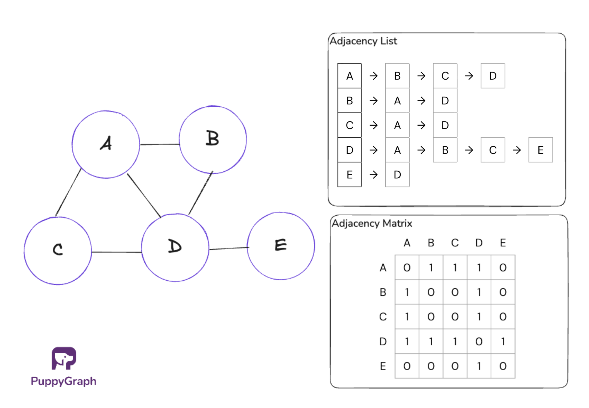
Sparse vs Dense Graphs

An important reason for the distinction between sparse and dense graphs is because it affects storage choice. In dense graphs, there are more edges, and matrices are recommended because checking an edge can be done in O(1) time, whereas lookup on a list is O(n). For sparse graphs, adjacency lists are recommended because they save space, and linear search for an edge is fine when edges are sparse.

The graph density is a point of consideration when deciding how to choose and optimize graph algorithms. Sometimes, the optimization fails when the density changes. Here we will see two examples: Prim’s algorithm for Minimum Spanning Tree (MST) and Dijkstra’s algorithm for shortest path algorithms.

MST algorithms find a subset of edges that connects all vertices (no cycles) with the minimum total weight. Prim’s algorithm includes a step that finds the minimum-weight edge from the visited vertices to the unvisited vertices. With a simple scanning implementation, the algorithm’s total time complexity is O(V²). Alternatively, using a priority queue to manage the minimum edge reduces the complexity to O(E log E). However, while this optimization is effective for sparse graphs, it can be less efficient than the simple implementation for dense graphs, where the priority queue becomes a burden.

Shortest path algorithms compute minimum-distance routes between nodes. Dijkstra’s algorithm requires selecting the unvisited vertex with the smallest tentative distance from the source at each step. A straightforward scanning approach results in a total time complexity of O(V²). By employing a priority queue to track the vertex with the minimum distance, the complexity can be reduced to O(E log V). For sparse graphs, this optimization is highly effective, but in dense graphs, the computational cost of managing the priority queue may outweigh the benefits, making the simpler scanning method more efficient.

Impact on Graph Performance

Graph databases excel at handling sparse data. Traversals stay narrow, filters stay selective, and planners avoid touching most of the graph. But when data begins to scale in complexity and size, that's when the cracks begin to show. Let’s look at where performance degrades and what to consider as graphs become denser and larger.

Performance Degradation

As a graph gets denser, edges outpace vertices, so each hop touches many more neighbors and the cost of traversals, variable-length matches, and algorithms climbs sharply. Dense pockets generate many near-duplicate paths, making counting and deduping expensive, while broad predicates match large neighborhoods and push the planner toward wide scans that repeat work. 

The problems with dense graphs don’t just stop there. With index-free adjacency, starting from a high-degree node pulls a huge neighbor list. If it doesn’t fit in cache, it evicts useful pages and slows later queries. With index-backed adjacency, dense regions become large posting lists and wide joins. Regardless of the internals, the effect is the same: more data per hop and more repeated work.

Scalability and Partitioning

In large, dense graphs, dividing the graph across multiple machines becomes harder. More edges mean more relationships that span partitions, so queries leave their “home” shard more often and pay for extra network hops. Supernodes and dense pockets also concentrate traffic on a few partitions, which reduces parallelism and makes tail latency worse.

Graph databases can be difficult to scale precisely because the data is hard to split cleanly. In a relational system you can often shard vertically or horizontally without breaking most queries. In a graph, dense and highly interconnected data makes it such that any cut risks severing many useful paths.

Storage and Memory

Dense graphs consume space quickly because edges dominate well before nodes do. Small per-edge properties multiply by a large E, inflating on-disk stores, indexes, stats, and logs. Retained history and parallel edges thicken neighborhoods further. Memory pressure rises in lockstep: large adjacency or posting lists expand the resident working set, caches need more pages to keep hit rates, and analytics that project subgraphs into memory scale with edges loaded, not just vertices. When the working set doesn’t fit, expect more page faults, longer warm-ups, and slower queries as hot regions reload.

Tools & Methods to Measure Node and Edge Counts

Graph Traversal

A plain traversal can tally nodes and edges on the fly. The core idea works with either DFS or BFS: keep a visited set to skip repeats, and either increment a node counter as you go or just use len(visited) at the end. For directed graphs, increment the edge counter for each traversed outgoing edge that passes your filters. For undirected graphs, avoid double counting by counting an edge only the first time you encounter it. 

Complexity is linear in the size of what you traverse: O(V + E).

SQL-Based Graph Analytics

Relational databases have evolved to model and query graph structures, allowing organizations to run meaningful graph analytics without retiring their existing infrastructure. In graph analytics, nodes represent entities. When modeling graphs in relational databases, these nodes become standard SQL tables. 

To give an example, let’s create a simple social video network graph. We have two core entity types that will serve as graph nodes:

• Users

CREATE TABLE users (
    id INT PRIMARY KEY,
    name VARCHAR(50) NOT NULL,
    created_at TIMESTAMP DEFAULT CURRENT_TIMESTAMP
);

• Videos

CREATE TABLE videos (
  id INT PRIMARY KEY,
  title VARCHAR(100) NOT NULL,
  duration_seconds INT NOT NULL,
  created_at TIMESTAMP DEFAULT CURRENT_TIMESTAMP
);

We’ll support two types of relationship here:

• Follows (user-to-user): 

CREATE TABLE follows (
  follower_id INT NOT NULL,
  followee_id INT NOT NULL,
  created_at TIMESTAMP DEFAULT CURRENT_TIMESTAMP,
  PRIMARY KEY (follower_id, followee_id),
  FOREIGN KEY (follower_id) REFERENCES users(id) ON DELETE CASCADE,
  FOREIGN KEY (followee_id) REFERENCES users(id) ON DELETE CASCADE
);

• Likes (user-to-video)

CREATE TABLE likes (
  user_id INT NOT NULL,
  video_id INT NOT NULL,
  created_at TIMESTAMP DEFAULT CURRENT_TIMESTAMP,
  PRIMARY KEY (user_id, video_id),
  FOREIGN KEY (user_id) REFERENCES users(id) ON DELETE CASCADE,
  FOREIGN KEY (video_id) REFERENCES videos(id) ON DELETE CASCADE
);

Once we populate the tables, we can simply sum up the entries in the node tables and edge tables to get the node and edge counts respectively:

• Node Count

WITH counts AS (
  SELECT COUNT(*) AS count FROM users
  UNION ALL
  SELECT COUNT(*) FROM videos
)
SELECT SUM(count) AS V FROM counts;

• Edge Count

WITH counts AS (
  SELECT COUNT(*) AS count FROM follows
  UNION ALL
  SELECT COUNT(*) FROM likes
)
SELECT SUM(count) AS E FROM counts;

While modelling a graph in SQL seems easy enough, the tradeoff shows up as soon as queries become more complex. Multi-hop questions become chains of self-joins or recursive CTEs. SQL graphs can quickly become hard to understand, with costly table joins slowing down performance.

Graph Databases

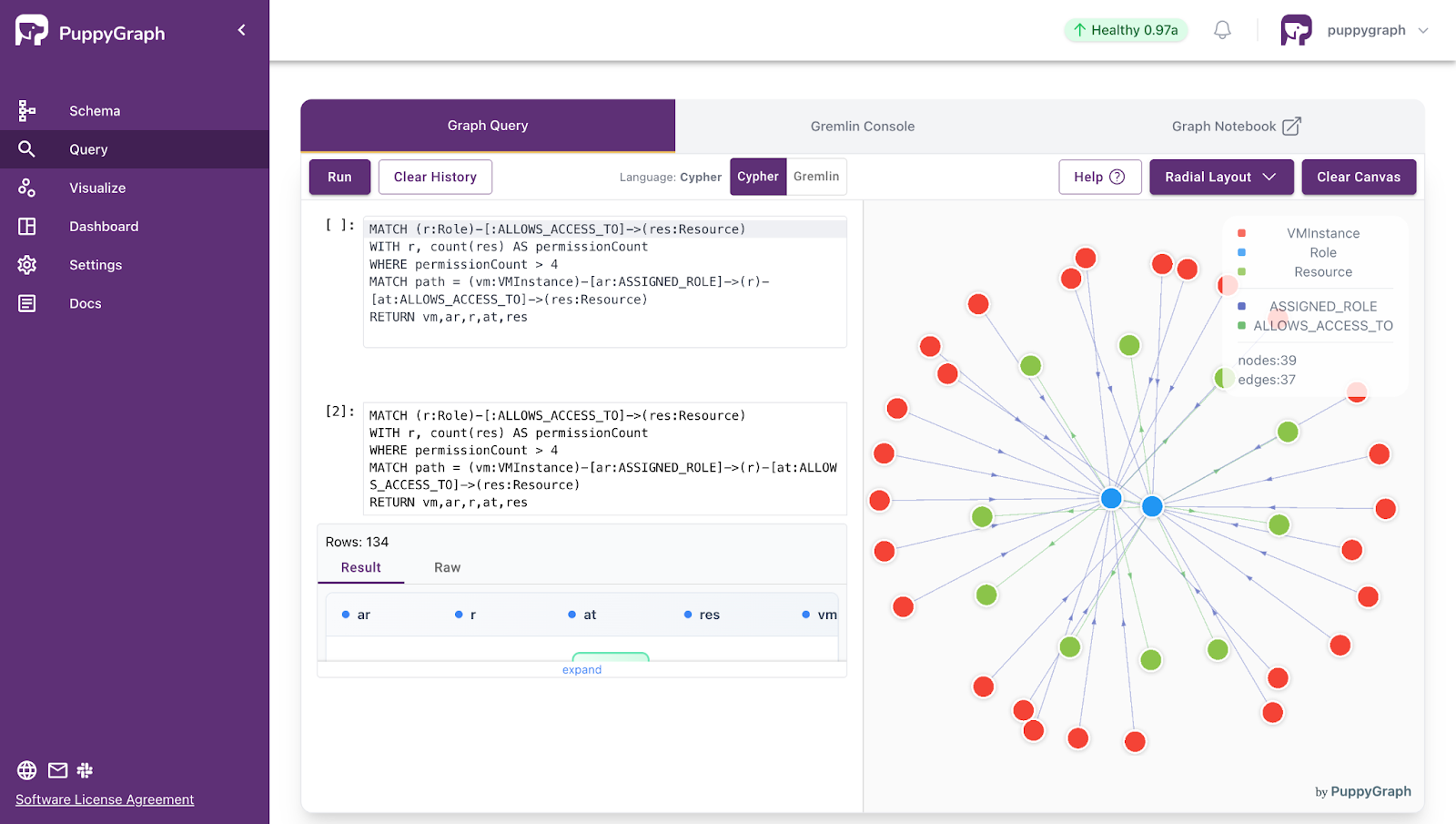
If you plan to run complex, multi-hop graph queries, a native graph database is a strong fit. The exact syntax depends on the language your database supports. Most graph databases also expose fast metadata or counters for totals and per-type counts, so these reads are usually quick. We’ll look at Cypher and Gremlin, two popular graph query languages. 

• Cypher

// Node count
MATCH (n) RETURN count(*);

// Edge Count
MATCH ()-[r]->() RETURN count(*);

• Gremlin

// Node count
g.V().count()

// Edge count
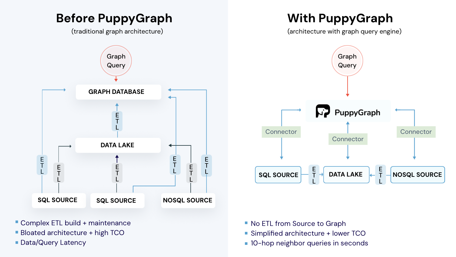
g.E().count()

But most organizations keep their source of truth in a relational system, so getting data into a graph database means building and maintaining ETL. That adds operational overhead and a second schema to keep in sync. It also introduces lag: batches or micro-batches create a freshness gap that can break real-time or near–real-time analytics. 

Graph Query Engines

SQL can model graphs, but multi-hop questions turn into long self-joins or recursive CTEs that are hard to read and slow to run. A separate graph database fixes the query shape but adds ETL, drift, and freshness gaps. Here’s where graph query engines really shine.

PuppyGraph is the first and only real time, zero-ETL graph query engine in the market, empowering data teams to query existing relational data stores as a unified graph model that can be deployed in under 10 minutes, bypassing traditional graph databases' cost, latency, and maintenance hurdles.

It seamlessly integrates with data lakes like Apache Iceberg, Apache Hudi, and Delta Lake, as well as databases including MySQL, PostgreSQL, and DuckDB, so you can query across multiple sources simultaneously.

Key PuppyGraph capabilities include:

• Zero ETL: PuppyGraph runs as a query engine on your existing relational databases and lakes. Skip pipeline builds, reduce fragility, and start querying as a graph in minutes.

• No Data Duplication: Query your data in place, eliminating the need to copy large datasets into a separate graph database. This ensures data consistency and leverages existing data access controls.

• Real Time Analysis: By querying live source data, analyses reflect the current state of the environment, mitigating the problem of relying on static, potentially outdated graph snapshots. PuppyGraph users report 6-hop queries across billions of edges in less than 3 seconds.

• Scalable Performance: PuppyGraph’s distributed compute engine scales with your cluster size. Run petabyte-scale workloads and deep traversals like 10-hop neighbors, and get answers back in seconds. This exceptional query performance is achieved through the use of parallel processing and vectorized evaluation technology. 

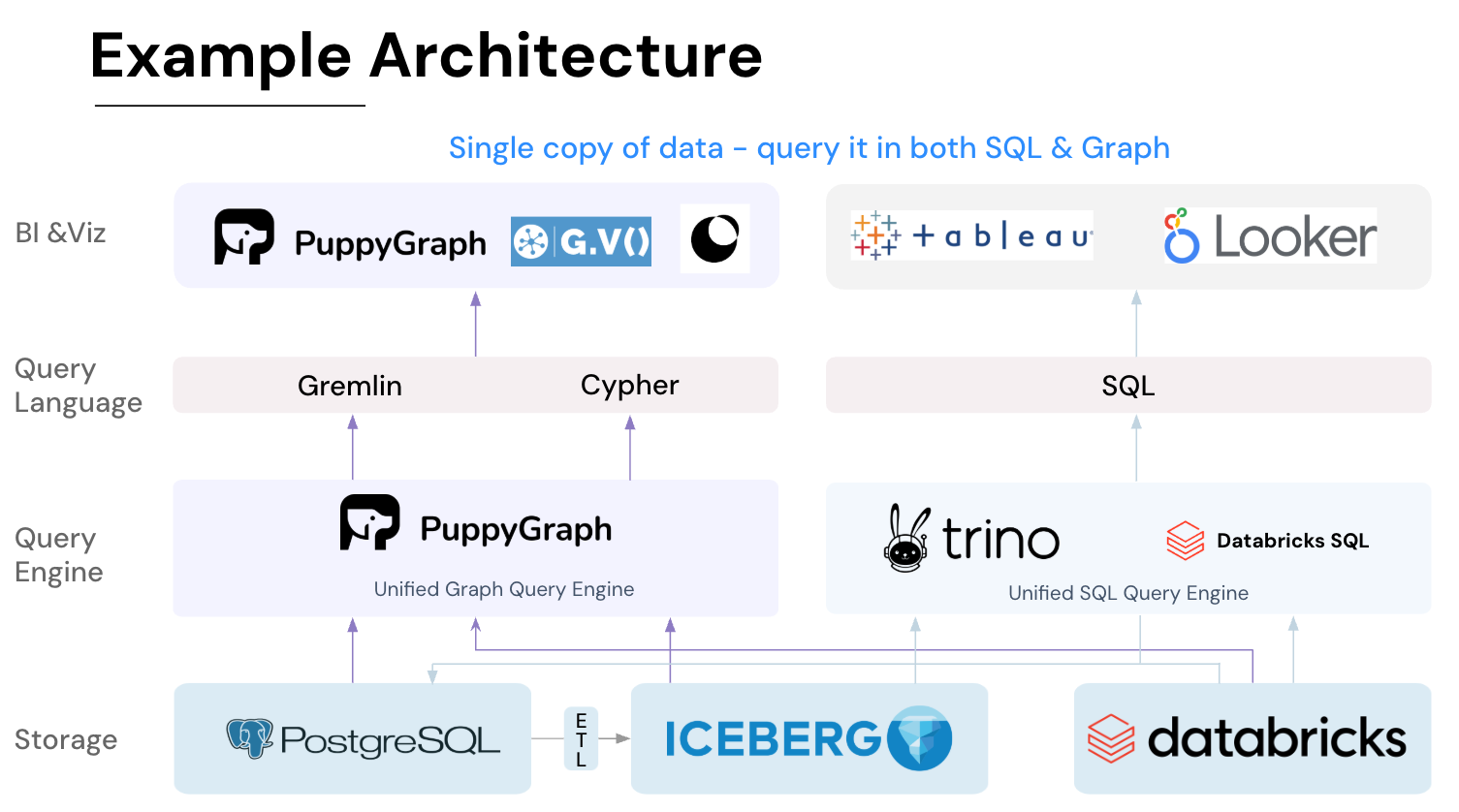
• Best of SQL and Graph: Because PuppyGraph queries your data in place, teams can use their existing SQL engines for tabular workloads and PuppyGraph for relationship-heavy analysis, all on the same source tables. No need to force every use case through a graph database or retrain teams on a new query language.

• Lower Total Cost of Ownership: Graph databases make you pay twice — once for pipelines, duplicated storage, and parallel governance, and again for the high-memory hardware needed to make them fast. PuppyGraph removes both costs by querying your lake directly with zero ETL and no second system to maintain. No massive RAM bills, no duplicated ACLs, and no extra infrastructure to secure.

• Flexible and Iterative Modeling: Using metadata driven schemas allows creating multiple graph views from the same underlying data. Models can be iterated upon quickly without rebuilding data pipelines, supporting agile analysis workflows.

• Standard Querying and Visualization: Support for standard graph query languages (openCypher, Gremlin) and integrated visualization tools helps analysts explore relationships intuitively and effectively.

• Proven at Enterprise Scale: PuppyGraph is already used by half of the top 20 cybersecurity companies, as well as engineering-driven enterprises like AMD and Coinbase. Whether it’s multi-hop security reasoning, asset intelligence, or deep relationship queries across massive datasets, these teams trust PuppyGraph to replace slow ETL pipelines and complex graph stacks with a simpler, faster architecture.

As data grows more complex, the most valuable insights often lie in how entities relate. PuppyGraph brings those insights to the surface, whether you’re modeling organizational networks, social introductions, fraud and cybersecurity graphs, or GraphRAG pipelines that trace knowledge provenance.

Deployment is simple: download the free Docker image, connect PuppyGraph to your existing data stores, define graph schemas, and start querying. PuppyGraph can be deployed via Docker, AWS AMI, GCP Marketplace, or within a VPC or data center for full data control.

Conclusion

Nodes tell you what exists. Edges tells you how it connects. Read them together to sanity-check data quality, spot where connectivity concentrates, and anticipate how queries will behave as graphs scale. Sparse graphs keep traversals tight, while dense pockets and supernodes raise cost, skew partitions, and inflate storage and memory. The right counts and a few lightweight ratios give you early warning before performance drifts.

If you’re working in SQL, multi-hop questions turn into long join chains. If you move data to a separate graph database, you inherit ETL and freshness gaps. A graph query engine lets you ask graph-shaped questions where your data already lives.

Want to try this without heavy lift? PuppyGraph lets you model and query your existing data as a graph in minutes. Start with our forever-free PuppyGraph Developer Edition, or book a demo to see real workloads end-to-end.