Graph Data Warehouse: Architecture, Benefits & Use Cases

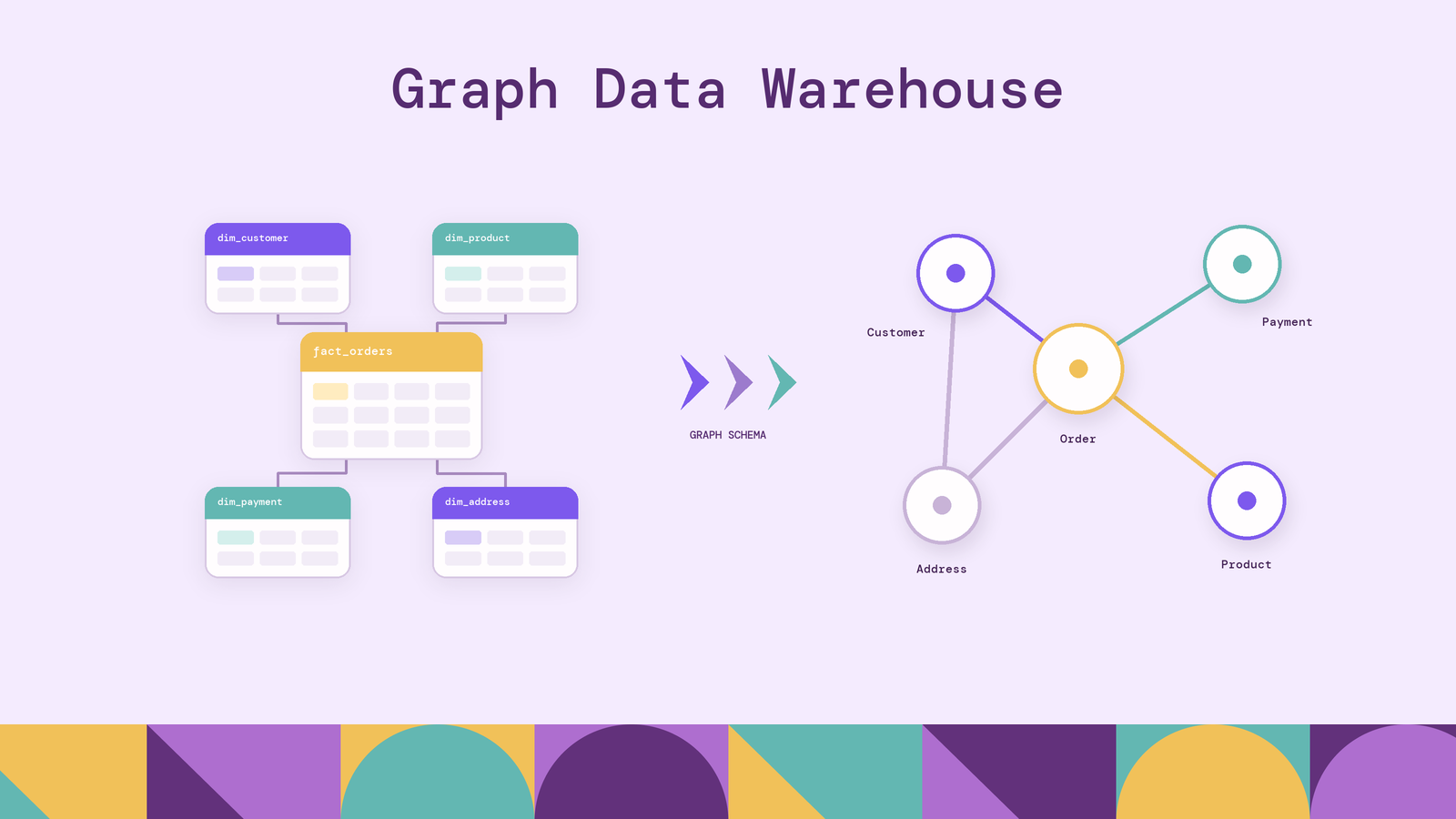
A data warehouse already knows which entities matter and how events connect them; its dimension and fact tables encode exactly that. What it cannot do is follow those connections for more than a few hops at a time. Which customers share a payment instrument with an account that charged back, which finished goods a supplier outage reaches through second-tier parts: in SQL each becomes a chain of self-joins whose depth is guessed before the query runs, and the usual remedy has been a separate graph database fed by one more pipeline.

This guide covers what a graph data warehouse is, how it works, the layers it is built from, how it compares with a traditional data warehouse and with a graph database, its benefits and use cases, and the practices that keep one useful.

What is a graph data warehouse?

A data warehouse is the central store where an organization’s data is integrated from its source systems, modeled into fact and dimension tables, and served to reporting and analytics through SQL. It is built for aggregation: totals by region, trends by month, drill-downs along known joins.

Some questions are about connections instead. Which accounts link to a flagged one through shared devices or payment instruments, which products a supplier failure reaches through two tiers of parts. These are graph queries: they follow relationships hop by hop, to a depth that is not known in advance. The warehouse holds the data for them, but SQL expresses each one as a chain of self-joins with the depth fixed before the query runs.

The established answer has been to load the relevant tables into a graph database and query there, at the cost of a pipeline, a refresh schedule, and a second copy to govern.

A graph data warehouse is a data warehouse that also serves graph queries directly over its own tables. A graph model is declared over the existing fact and dimension tables, with dimension tables as nodes and fact and bridge tables as edges, and queries are written in a graph language that follows those edges to whatever depth the answer needs. The warehouse stays the system of record and the tables do not move; the graph is another way of reading them, with no copy loaded anywhere. This is the arrangement PuppyGraph implements, and the rest of this guide describes it in general terms before returning to the product.

The reason this works so well is that the warehouse has already done the hardest part of building a graph. Bill Inmon’s definition in Building the Data Warehouse calls a warehouse subject-oriented and integrated: organized around business entities, with each customer, product, or account reconciled to one identity across every source that mentions it. That is entity resolution, the step that consumes most of a graph project, finished before the project starts. Kimball’s dimensional modeling then records every event as a fact table row carrying a foreign key to each dimension it involves, which is a relationship between resolved entities, stored and governed. Nodes with settled identities and edges recorded between them are what a graph is made of, and a well-built warehouse holds both before any graph is declared. The graph model does not add information; it makes what the warehouse already knows queryable in the shape it already has.

How does a graph data warehouse work?

Nothing about the warehouse’s tables, loads, or SQL workloads changes. A graph data warehouse adds a mapping and an execution path over the modeled layer.

The mapping follows the dimensional model. A dim_customer table becomes a Customer node type keyed by its surrogate key, with its columns as properties. A fact table becomes edges: a row in fact_orders carrying customer_key, payment_key, and address_key yields a PAID_WITH edge from customer to payment instrument and a SHIPPED_TO edge from customer to address, with order date and amount as edge properties. Bridge tables, which already hold many-to-many relationships, map to edges directly. A fact that links many dimensions at once can instead become an event node with one edge per dimension, preserving the grain.

Queries arrive in graph vocabulary. The pattern below asks which customers are within two hops of a charged-back account through a shared payment instrument or shipping address, without deciding in advance which link type or how many of them the connection runs through:

MATCH (flagged:Customer {risk_flag: 'chargeback'})-[:PAID_WITH|SHIPPED_TO*1..2]-(c:Customer)
WHERE c <> flagged
RETURN c.customer_id, count(DISTINCT flagged) AS linked_flagged
ORDER BY linked_flagged DESC

The engine reads through the warehouse’s SQL interface. A warehouse's native tables sit in the platform's own internal format, reachable through its query layer rather than as files, so the graph engine does not read storage directly; it issues only simple projection and filter SQL to the warehouse and computes the traversal in its own engine, the query shape a columnar warehouse serves well.

Results come back inside the same perimeter. The reads are ordinary warehouse queries issued under a warehouse role, so the access control, masking, and audit logging attached to the tables apply to the traversal.

A new relationship question therefore costs a query rather than a project: no extract, no load, and no second schema to keep aligned with the one the BI tools use.

Graph data warehouse architecture

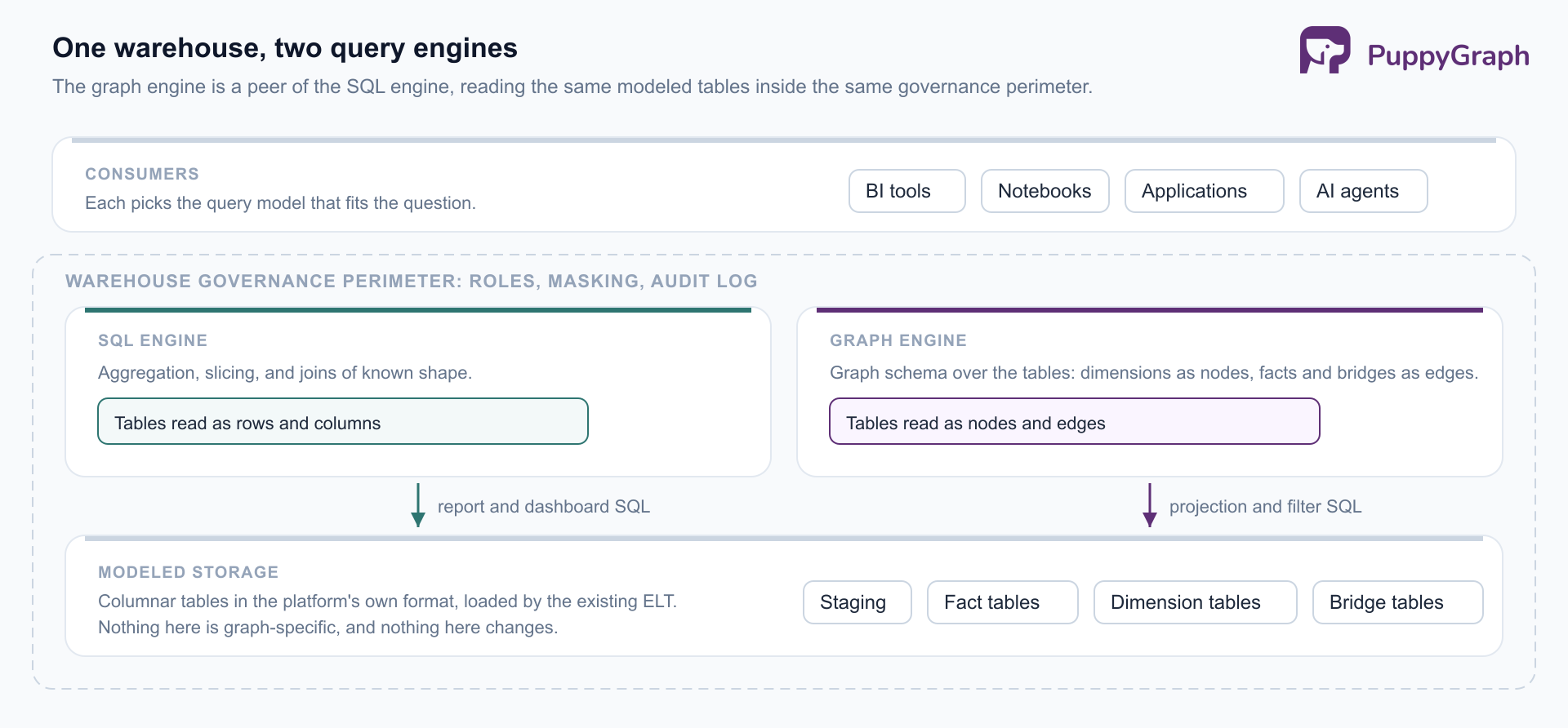
A graph data warehouse is the standard warehouse stack with one additional peer in the compute layer.

Modeled storage. The warehouse database itself: staging areas, then partitioned columnar tables holding the facts and dimensions, in the platform’s own format. Nothing here is graph-specific, and nothing here changes.

Warehouse compute. The MPP SQL engine that serves dashboards, reports, and transformations. Cloud platforms separate it from storage so that several compute clusters can serve different workloads over the same tables; Snowflake’s architecture describes a central storage layer with independent virtual warehouses reading from it. That separation makes room for a second engine.

Graph compute and the graph schema. The layer that distinguishes the architecture. It holds the mapping from tables to node and edge types, compiles a graph query into a plan of node and edge operators that runs in its own engine, reads the tables through simple projection and filter SQL, and scales on its own capacity. It is a peer of the SQL engine rather than a consumer downstream of it, because both read the modeled tables directly. In PuppyGraph this layer is the product: the mapping, the traversal engine, and its own compute, deployed beside the warehouse.

Metadata and governance. The warehouse’s catalog, roles, masking policies, and audit log. The graph engine authenticates as a warehouse principal, so a traversal sees what that principal sees.

Consumers. BI tools, notebooks, applications, and increasingly AI agents, each choosing the query model that fits the question.

Graph data warehouse vs. traditional data warehouse

A graph data warehouse is not a replacement for a traditional data warehouse. It is one with a second query model over the same tables, so the comparison is about what that access path adds.

Adopting the pattern does not fork the platform decision, the modeling methodology, or the security model. Storage, loads, the dimensional model, and governance stay as they are; what is added is an engine that reads the same tables with a different execution strategy. That also sets the boundary: if the analytical questions are aggregations over joins of known shape, the star schema was designed for exactly that work and the graph layer earns nothing. It earns its place when the answer depends on how far the connections reach.

Graph data warehouse vs. graph database

The sharper comparison is with a dedicated graph database, the incumbent answer to the same questions. The two differ less in what a query can express than in where the graph lives and what keeping it true costs. The table takes the deployment this article is about, where the warehouse is the system of record and the graph database would hold a copy of it.

A graph database is a system of record built for graph-shaped writes and low-latency lookups under application load, a workload the warehouse has no answer for. A graph data warehouse addresses the other case, where the data arrives and is modeled as tables and needs to be traversed analytically. The failure it removes is the copy: drift, load lag, schema changes that reach one system before the other, and a second set of access policies to keep honest.

Benefits of a graph data warehouse

The modeling is already done. Entity resolution is the expensive prerequisite of any graph project, and a warehouse’s conformed dimensions are that work, completed. A customer has one surrogate key across every fact table that references it, so the mapping to nodes and edges is a declaration over keys that already agree.

No second copy to keep in sync. The recurring cost of a graph project is the pipeline that keeps the graph current and the team that owns it. Removing the copy removes the drift and the pipeline together.

One governance perimeter. Roles, masking, and audit stay attached to the tables. Financial and customer data are common graph workloads, and duplicating them into a system with its own permission model is the kind of exception auditors ask about.

Relationship questions without pre-planned join depth. A variable-length path states the question in one pattern. In SQL the same question is either a chain of self-joins with the depth fixed in advance, or a recursive CTE that gets the answer but carries its own cycle guards, depth caps, and cost that climbs with each level. That changes what analysts can ask casually, not only how fast the answer arrives.

Graph data warehouse use cases

Fraud and anti-money-laundering. Fraud rings are defined by attributes shared across accounts (devices, addresses, payment instruments) and by circular transaction flows that appear only several hops out. Both are traversals over the transaction facts and customer dimensions the warehouse already holds.

Customer 360. A customer dimension conformed across sales, support, and marketing is one node type, and the fact tables around it are the edges. Households, shared accounts, referral chains, and account hierarchies become paths over tables the warehouse already holds.

Supply chain and dependency risk. Suppliers, parts, plants, and shipments form a multi-tier network, and the question after a disruption is which finished goods it reaches through second- and third-tier dependencies.

Knowledge graphs and AI agents. A knowledge graph is a semantic model of a domain, and a warehouse’s dimensional model is most of one already. Declared as a graph schema, it becomes an ontology that applies at query time over live data, and it gives an AI agent a vocabulary of entities and relationships to query through, with the meaning of each table stated in the model.

The shared trait is data that arrives as tables, is modeled for reporting, and is only sometimes asked a relationship question. That is the profile where a permanent second copy is hardest to justify.

Graph data warehouse best practices

Map from the grain, not from every foreign key. A fact table’s grain says what one row means, and that decides whether the row is an edge between two dimensions or an event node connected to several. Mapping every foreign key to an edge produces a graph that is technically correct and semantically useless.

Respect slowly changing dimensions. A type 2 dimension holds several rows per entity, each with a validity window. Map the durable business key to the node and carry the version rows as time-scoped properties or edges, or the traversal will split one customer into as many nodes as it has address changes.

Design for supernodes. A shared IP address, a popular product, or a house account turns one hop into an explosion. Bound path length, filter edge types early, and model high-degree entities deliberately.

Check governance through the mapping. Masking and row-level policies are written over tables. Once a table is a node type, verify that no property or path exposes what a policy hides, especially where the graph joins tables from different trust boundaries.

Evaluate the engine at real depth. The mapping decides what the graph means; the engine decides how a traversal runs against columnar tables laid out for wide scans, and that behavior only shows at depth. Test a candidate on the deepest query the team actually runs, with realistic fan-out, before committing to it.

PuppyGraph is built for the path this guide describes: the graph is declared over the warehouse’s tables and queried there, with nothing loaded out. It compiles a graph query into a plan of node and edge operators that runs in its own distributed engine, issuing only simple projection and filter SQL to the warehouse. Because the query is represented as graph operators end to end, the engine optimizes specifically for multi-hop traversals and pattern matching, which is where its traversal performance comes from. The same engine reads data lakes and lakehouses, including direct reads of open table formats like Iceberg and Delta Lake, and queries run in openCypher and Gremlin. The graph schema it declares over the warehouse’s tables doubles as an ontology: queries are validated against it before execution, so a reference to an entity or relationship the model does not define is rejected with structured feedback in domain terms rather than a stack trace.

Conclusion

The warehouse was built to integrate an organization’s data once, model it deliberately, and serve every question afterward from the same tables. A graph data warehouse applies that premise to the questions a warehouse serves least well: how entities connect, how far a path reaches, and what a change touches downstream. The dimensional model already names the entities and records the events between them; the graph is a way of reading that model in place, which is what keeps it current and governed. As AI agents become a major consumer of warehouse data, the same layer gives them a model of what the tables mean.

Try the forever-free PuppyGraph Developer Edition and book a demo with the team to see how openCypher and Gremlin queries traverse warehouse and lakehouse tables, with no graph-specific ETL, turning the dimensions and facts your warehouse already models into a graph.