The article

Query your table as a graph.Petabytes. Subsecond. No data movement.
In a SQL self join, the important decision is which rows belong together: an employee with their manager, two colleagues in the same team, or successive levels in a reporting chain. That decision determines whether a query returns the relationships you intended or a misleading set of matches.
This guide explains SQL self join syntax through one employee dataset, including INNER JOIN and LEFT JOIN examples, multiple conditions, hierarchical queries, and practical optimization. The examples use PostgreSQL; recursive-query syntax and plan-inspection commands vary across databases.
What is a self join in SQL?
A self join joins a table to itself so that a query can compare or combine values from different rows in that table. Each reference receives a distinct alias, giving the same underlying data two roles. PostgreSQL's join tutorial illustrates this pattern using two references to one table.
There is no separate SELF JOIN keyword. You use ordinary join syntax, such as INNER JOIN or LEFT JOIN, and name the same table on both sides. “Self” identifies where the inputs come from; the join type determines what happens to unmatched rows.
Common applications include attaching manager names to employees, comparing products within a category, identifying pairs of records with matching attributes, and finding a category's parent. A self join does not require a hierarchy or even a foreign key. Its condition can compare any suitable columns, including numeric ranges or dates.
The useful starting point is to describe each role in plain language. Employee and manager imply a different relationship from employee and colleague, even though both queries read the employee table twice.
How does a self join work?
Consider this fictional directory. Salaries are annual amounts in the same currency.
| employee_id | employee_name | manager_id | department | salary |
|---|---|---|---|---|
| 1 | Maya | NULL | Executive | 180000 |
| 2 | Luis | 1 | Engineering | 150000 |
| 3 | Priya | 1 | Operations | 145000 |
| 4 | Noah | 2 | Engineering | 120000 |
| 5 | Amina | 2 | Engineering | 160000 |
| 6 | Chen | 3 | Operations | 110000 |
| 7 | Elena | 4 | Engineering | 100000 |
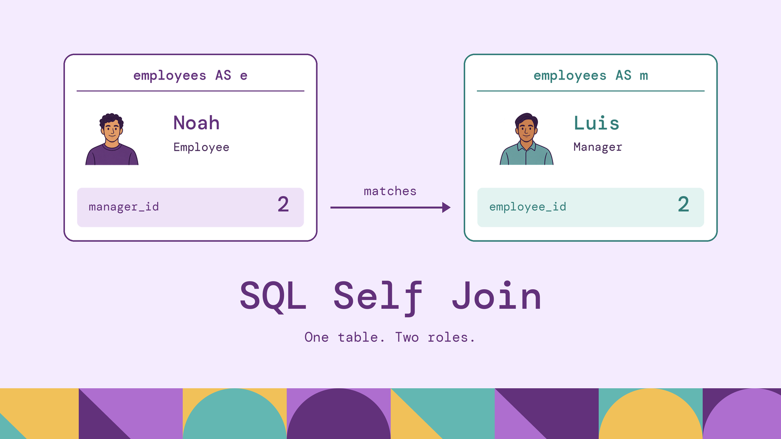
For a manager lookup, call the employee reference e and the manager reference m. The condition e.manager_id = m.employee_id matches Noah's manager_id of 2 to Luis's employee_id of 2. The result can then contain Noah's name from e and Luis's name from m.
The aliases do not create stored copies of the table. They identify independent references within the query. Thinking through candidate row pairs explains the result, but the database chooses its physical execution plan; it need not compare every possible pair.
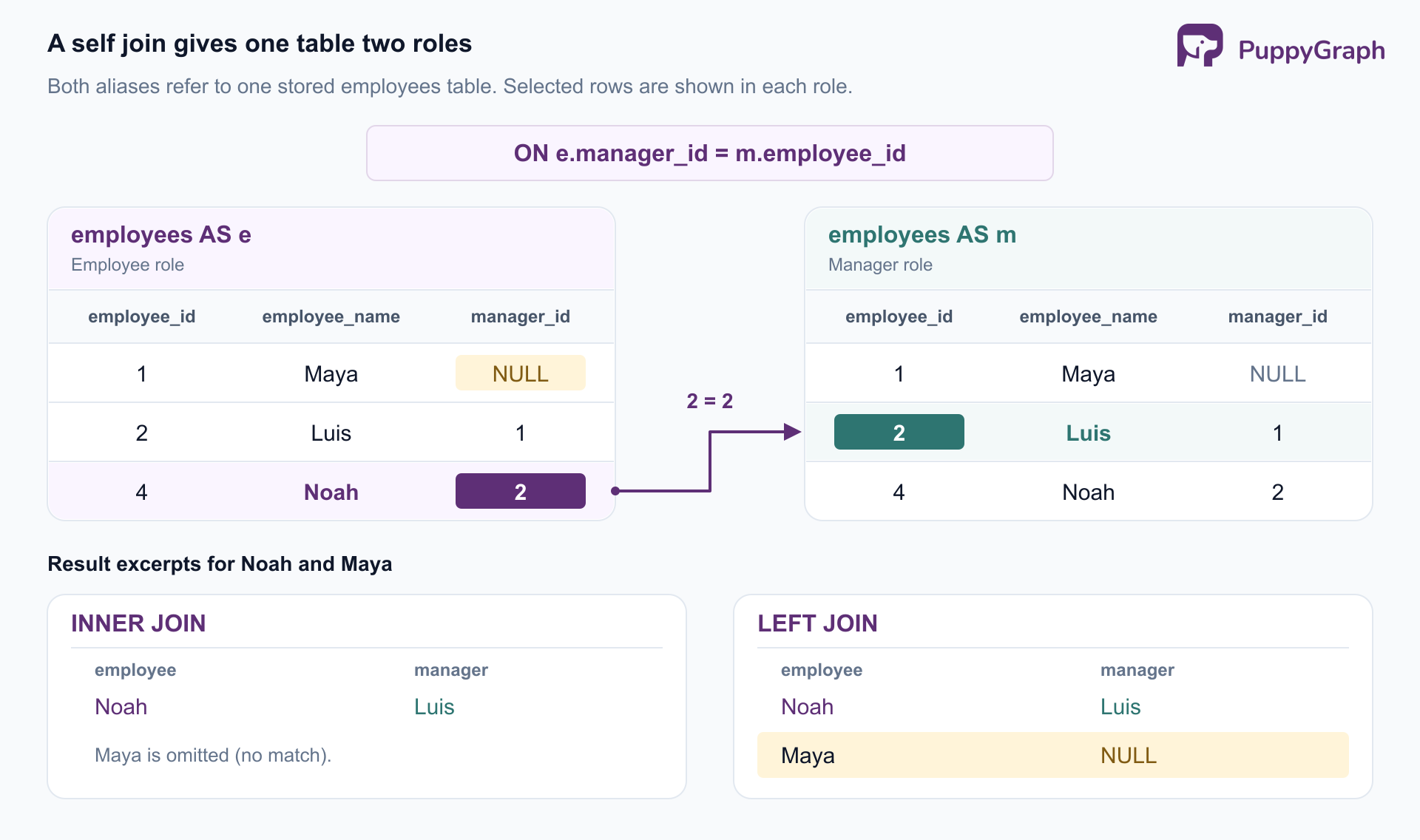
Figure: Aliases give one table two roles; the join condition matches the rows. LEFT JOIN also preserves employees such as Maya who have no matching manager.
Maya has no manager. With an inner join she contributes no employee-side result. With a left join she remains, with NULL in the manager fields. Decide whether such unmatched rows belong in the answer before choosing the join type.
SQL self join syntax
Create the example table and load its rows:
CREATE TABLE employees (
    employee_id INTEGER PRIMARY KEY,
    employee_name VARCHAR(50) NOT NULL,
    manager_id INTEGER REFERENCES employees(employee_id),
    department VARCHAR(50) NOT NULL,
    salary INTEGER NOT NULL
);

INSERT INTO employees VALUES
    (1, 'Maya', NULL, 'Executive', 180000),
    (2, 'Luis',    1, 'Engineering', 150000),
    (3, 'Priya',   1, 'Operations', 145000),
    (4, 'Noah',    2, 'Engineering', 120000),
    (5, 'Amina',   2, 'Engineering', 160000),
    (6, 'Chen',    3, 'Operations', 110000),
    (7, 'Elena',   4, 'Engineering', 100000);
The self-referential foreign key ensures that each non-null manager_id identifies an existing employee. It protects the data independently of how you query it.
The self join has this form:
SELECT e.employee_name, m.employee_name AS manager_name
FROM employees AS e
JOIN employees AS m
  ON e.manager_id = m.employee_id;
FROM introduces the employee role; JOIN introduces the manager role. ON defines the relationship between them. The table aliases qualify column references, while AS manager_name labels an output column. Plain JOIN means INNER JOIN here.
Use meaningful aliases and qualify columns consistently. A bare employee_name is ambiguous because both references expose that column. Explicit output columns also make the intended relationship easier to review than SELECT *, which returns both sets of fields.
SQL self join examples
Find employees and their managers with INNER JOIN. This query returns employees whose manager exists:
SELECT e.employee_name AS employee,
       m.employee_name AS manager
FROM employees AS e
INNER JOIN employees AS m ON e.manager_id = m.employee_id
ORDER BY e.employee_id;| employee | manager |
|---|---|
| Luis | Maya |
| Priya | Maya |
| Noah | Luis |
| Amina | Luis |
| Chen | Priya |
| Elena | Noah |
Maya appears in the manager column but has no row in the employee column. The join treats her differently in each role. Luis likewise appears as an employee reporting to Maya and as the manager of Noah and Amina.
Keep every employee with LEFT JOIN. Change the join type when the report must include people without managers:
SELECT e.employee_name AS employee,
       m.employee_name AS manager
FROM employees AS e
LEFT JOIN employees AS m ON e.manager_id = m.employee_id
ORDER BY e.employee_id;
The result contains the same six matches plus Maya | NULL at the beginning. All seven employees remain. In this schema, the manager's primary key permits at most one match per employee, so this query returns exactly one row per employee. A left join on a non-unique column could return several matches instead.
Compare an employee's salary with their manager's. Once the rows are paired, both salaries are available to a filter:
SELECT e.employee_name AS employee,
       e.salary AS employee_salary,
       m.employee_name AS manager,
       m.salary AS manager_salary
FROM employees AS e
JOIN employees AS m ON e.manager_id = m.employee_id
WHERE e.salary > m.salary
ORDER BY e.employee_id;
The single result pairs Amina, earning 160000, with her manager Luis, earning 150000. The join establishes the reporting relationship; the filter compares the two salaries. Comparing every employee with every higher-paid employee would answer a different question.
These examples share one relationship condition. Changing the join type changes which employees survive; changing the filter changes which matched relationships qualify.
Self join with multiple conditions
A join condition can combine several requirements. To find pairs of employees who share both a department and a manager, use:
SELECT a.employee_name AS employee_1,
       b.employee_name AS employee_2
FROM employees AS a
JOIN employees AS b
  ON a.department = b.department
 AND a.manager_id = b.manager_id
 AND a.employee_id < b.employee_id
ORDER BY a.employee_id, b.employee_id;
The result is Noah | Amina. Luis and Priya share a manager but have different departments, so they fail the first condition. Elena belongs to Engineering but reports to Noah, so she does not pair with Amina.
The ID comparison does two jobs: it excludes pairing a row with itself and keeps only one ordering of each pair. Using <> would exclude self-pairs but return both Noah | Amina and Amina | Noah. Use < when the pair is unordered; use a directional condition when each row has a distinct role.
Nulls need deliberate treatment. Under SQL's comparison rules, NULL = NULL is not true. Two employees with no manager therefore do not qualify as sharing a manager through this equality condition. That is often appropriate: two missing relationships do not establish a shared supervisor.
When combining AND and OR, parenthesize alternatives so that requirements such as excluding self-pairs apply to the whole condition. Each condition should correspond to a relationship rule you can explain from the data.
How to use self joins for hierarchical data
A parent ID stored on each row is an adjacency-list representation of a hierarchy. Each additional self join can follow another level. To find Elena, her manager, and her manager's manager:
SELECT e.employee_name AS employee,
       m.employee_name AS manager,
       gm.employee_name AS managers_manager
FROM employees AS e
LEFT JOIN employees AS m ON e.manager_id = m.employee_id
LEFT JOIN employees AS gm ON m.manager_id = gm.employee_id
WHERE e.employee_id = 7;
This returns Elena | Noah | Luis. The query stops at two reporting links because it contains two joins. Another alias would extend it by one level. Left joins retain the starting employee even if the chain ends earlier.
When the required depth depends on the data, use a recursive CTE. This PostgreSQL query finds Luis's direct and indirect reports:
WITH RECURSIVE team AS (
    SELECT employee_id, employee_name, 0 AS depth
    FROM employees
    WHERE employee_id = 2

    UNION ALL

    SELECT e.employee_id, e.employee_name, t.depth + 1
    FROM employees AS e
    JOIN team AS t ON e.manager_id = t.employee_id
)
CYCLE employee_id SET is_cycle USING path
SELECT employee_name, depth
FROM team
WHERE depth > 0 AND NOT is_cycle
ORDER BY depth, employee_id;
The anchor selects Luis at depth zero. The recursive term finds employees reporting to the previous iteration's employees. It returns Noah and Amina at depth one, then Elena at depth two; the outer filter excludes Luis.
CYCLE detects a repeated employee on a path, stops expanding that cyclic branch, and marks the repeated row. The final filter removes marked rows. A depth limit can bound a business question, but it can also omit deeper descendants; it is not equivalent to finding the complete hierarchy. Other databases use different cycle-handling syntax.
Choose fixed joins for a fixed number of levels and recursion for descendants at arbitrary depth. The recursive join guide develops the latter pattern further.
Self join performance and optimization
A self join's cost depends on its predicate, matching-row counts, indexes, and chosen execution plan. A manager lookup and an all-pairs comparison have very different workloads even though both reference one table twice.
Estimate the result size. A join to a unique manager ID produces at most one match per employee. By contrast, pairing every member of a group with every other member produces n × (n - 1) / 2 unordered pairs. An index cannot remove the cost of returning relationships the query explicitly requests. Restrict the scope to the departments or employees the report actually needs.
Index the lookup direction. PostgreSQL creates an index for the employee_id primary key. Looking up reports by manager uses the other side of the relationship, so a candidate index is:
CREATE INDEX employees_manager_id_idx
ON employees (manager_id);
PostgreSQL does not automatically index referencing columns merely because they have a foreign key constraint. The new index can help searches by manager, but the planner may prefer a scan, especially for a small table. For frequent queries combining department and manager equality, evaluate a multicolumn index against the actual workload.
Inspect the plan with representative data. PostgreSQL's EXPLAIN ANALYZE executes the query and reports actual row counts alongside estimates:
EXPLAIN (ANALYZE, BUFFERS)
SELECT e.employee_name, m.employee_name AS manager
FROM employees AS e
JOIN employees AS m ON e.manager_id = m.employee_id
WHERE e.department = 'Engineering';
Look for large estimate errors, repeated work, and expensive intermediate results. A sequential scan of this seven-row fixture is reasonable. It cannot establish how the query will behave against a large directory with a different distribution of departments and managers.
Ask for only the result you need. If the question is whether an employee has any direct reports, EXISTS expresses that without returning one row per report. Pair generation followed by DISTINCT can do unnecessary work when the application only needs a yes-or-no test.
For workloads centered on reporting paths across many levels, a graph model provides another way to express those relationships over the existing data.
PuppyGraph is the first and only zero-ETL graph query engine that lets you query existing relational data as a graph. It is a distributed graph query engine that queries tables in place in SQL databases, data warehouses, and data lakes or lakehouses, including direct reads of Iceberg and Delta Lake, without ETL into a separate graph database. Connect the sources, define a graph schema mapping tables to nodes and edges, and query with openCypher or Gremlin; the same employee rows can represent employees and reporting relationships while remaining queryable with SQL.
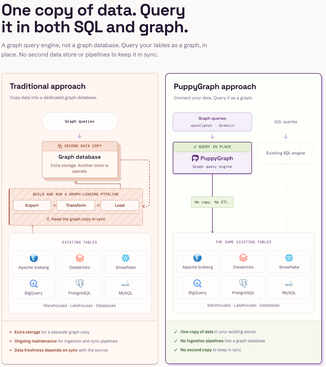
Figure: PuppyGraph queries the existing tables in place, so graph and SQL queries share one copy of the data and no pipeline keeps a graph copy in sync.
Figure: Companies that use PuppyGraph.
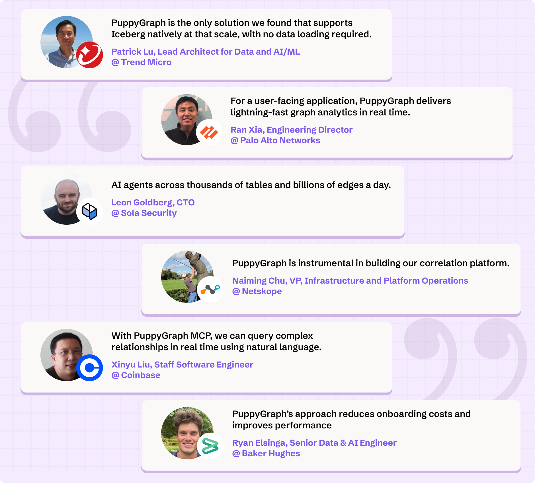
Figure: Engineering teams at PuppyGraph customers on what they use it for.
Mistakes when using SQL self joins
Reversing the roles. e.manager_id = m.employee_id looks up each employee's manager. e.employee_id = m.manager_id finds people reporting to e, despite the alias names. Trace one known relationship, such as Noah reporting to Luis, before trusting a larger result.
Filtering away outer rows. After a left join, WHERE m.department = 'Engineering' removes unmatched employees because their manager fields are null. If the intent is to retain every employee but attach only Engineering managers, put that condition in ON. PostgreSQL's table-expression documentation demonstrates why those placements produce different outer-join results.
Hiding a wrong predicate with DISTINCT. Matching employees on department alone creates all qualifying pairs within each department. Multiple matches may be correct, or they may expose a missing condition. Check the expected relationship and its uniqueness before collapsing rows. For unordered pairs, impose an ordering on unique IDs.
Assuming valid references guarantee a tree. A foreign key prevents a manager ID from pointing to a missing employee, but it does not prevent someone from managing themselves or a cycle between several employees. Enforce hierarchy rules when writing data and protect recursive queries against cycles. In an unconstrained imported table, also distinguish a legitimate null manager from a non-null manager ID with no matching row.
Conclusion
A SQL self join assigns different roles to rows from the same table. Correct results depend on the relationship condition, the treatment of unmatched rows, and the number of matches each row can produce. Use INNER JOIN for matches, LEFT JOIN to preserve the starting rows, and ordered IDs to produce unique unordered pairs. Fixed join chains handle known levels; recursive CTEs handle variable depth.
Try the forever-free PuppyGraph Developer Edition and book a demo with the team to see how openCypher and Gremlin queries follow relationships across warehouse and lakehouse tables, with no graph-specific ETL, as reporting questions extend beyond direct managers.