SQL Execution Plan: How It Works and How to Read It
- Hao WuSoftware Engineer
The guide

Query your table as a graph.Petabytes. Subsecond. No data movement.
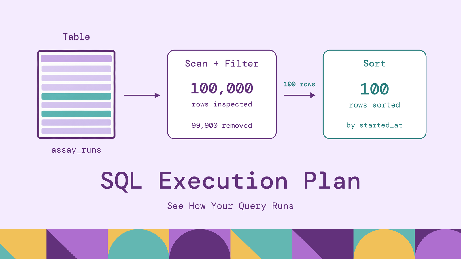
A slow SQL query often spends its time doing work that its text barely suggests: reading discarded rows, repeating lookups, or sorting an unexpectedly large intermediate result. An execution plan makes that work visible, so a proposed optimization has something concrete to explain.
This guide covers plan generation, operators, and a practical reading method. A PostgreSQL example follows a laboratory's failed assay runs from an initial table scan to indexed access, with SQL Server and MySQL instructions alongside it.
What is an execution plan in SQL?
A SQL execution plan describes the physical operations a database chooses to produce a query's result. It identifies access methods, join algorithms, filters, and operations such as sorting and aggregation. A graphical plan and a text plan can represent the same underlying work.
SQL specifies the result you want. The plan determines how to obtain it. An inner join, for example, does not require one particular join algorithm or physical input order. The optimizer evaluates alternatives that preserve the query's meaning. PostgreSQL's planner documentation describes this search over access paths and join strategies.
The plan is therefore specific to an engine and planning context. Identical SQL can produce different plans when indexes, statistics, parameters, or settings differ.
How does a SQL execution plan work?
PostgreSQL's query processing stages provide a useful model. The parser checks the statement and constructs a query tree. Rewriting can expand a view into its underlying query. The planner then selects physical operations, and the executor processes the resulting plan.
The planner estimates how many rows each operation will produce and the work required to process them. Available indexes and data statistics influence these estimates. Filtering a large input early can change the cost of every operation above it.
Optimization has its own budget. An engine need not examine every theoretically possible plan before choosing one; complex join searches can use heuristics. A chosen plan reflects the alternatives considered and the estimates available, rather than a guarantee of minimum elapsed time.
Execution follows the plan's dependencies. In PostgreSQL's executor, parent nodes request rows from their children. Some operations can return rows incrementally; a conventional sort needs its input before returning sorted output.
Key components of an execution plan
Read a plan as connected operators with properties attached:
Operators and inputs. A scan produces rows, a join combines inputs, and a sort orders them. Indentation or connecting arrows show which operator consumes another's output.
Estimated rows and width. PostgreSQL's rows estimate describes rows emitted by a node, not all rows inspected. width estimates the average output row size in bytes. Both help explain the volume passed downstream.
Estimated cost. PostgreSQL prints startup and total cost as cost=start..total. These are planner units, not milliseconds. Parent costs include child work, so adding every displayed cost double-counts that work. The official EXPLAIN guide defines these fields.
Predicates and runtime evidence. Conditions show where filtering occurs. An analyzed plan adds measurements such as actual rows and execution counts. PostgreSQL's BUFFERS option reports buffer activity: a shared hit finds a block in PostgreSQL's cache, while a shared read brings it into that cache. A read may still be served by the operating system's cache.
Types of SQL execution plans
The main distinction concerns collection. An estimated plan shows what the database intends to execute without running the statement. An actual plan includes observations from execution. SQL Server also offers Live Query Statistics, which exposes progress while a query runs; those counts remain incomplete until the work finishes.
Display format is a separate choice. Text is convenient for copying into an investigation. Graphical views make dependencies easier to inspect. Structured formats support automated comparisons. PostgreSQL offers JSON, XML, and YAML alongside text.
A graphical display does not automatically contain actual measurements. Check how the plan was collected before treating a number as observed behavior.
How to generate an execution plan in SQL
For PostgreSQL, run this deterministic fixture in a scratch database. It creates 100,000 synthetic assay runs, with timestamps stored without a time zone:
CREATE TABLE assay_runs AS
SELECT g AS run_id,
       1 + (g % 5000) AS sample_id,
       TIMESTAMP '2026-10-01'
         + ((g - 1) / 1000) * INTERVAL '1 day'
         + ((g - 1) % 1000) * INTERVAL '1 second' AS started_at,
       CASE WHEN g % 10 = 0 THEN 'failed'
            ELSE 'passed' END AS result_status
FROM generate_series(1, 100000) AS g;
ANALYZE assay_runs;
Find failed runs from one day and collect a plan:
EXPLAIN (ANALYZE, BUFFERS, TIMING OFF)
SELECT run_id, sample_id, started_at
FROM assay_runs
WHERE result_status = 'failed'
  AND started_at::date = DATE '2026-10-01'
ORDER BY started_at;
Plain EXPLAIN produces estimates. Adding ANALYZE executes the query. Here, TIMING OFF retains row counts and total execution time while avoiding per-node clock measurements. Remember that analyzing a data-changing statement executes its changes too.
In SQL Server Management Studio, select Query → Display Estimated Execution Plan for an estimated plan. Select Query → Include Actual Execution Plan, then execute the statement, for runtime information. SQL Server also supports SET SHOWPLAN_XML and SET STATISTICS XML, respectively.
For MySQL 8.4, use EXPLAIN FORMAT=TREE SELECT ... for estimates or EXPLAIN ANALYZE FORMAT=TREE SELECT ... to execute and measure a query. These are command patterns; supply your query after the prefix.
How to read and interpret an execution plan
The PostgreSQL 16 run produced this excerpt, with planning and total timing lines omitted:
Sort  (cost=2391.38..2391.50 rows=49 width=16) (actual rows=100 loops=1)
  Sort Key: started_at
  Sort Method: quicksort  Memory: 28kB
  Buffers: shared hit=640
  ->  Seq Scan on assay_runs  (cost=0.00..2390.00 rows=49 width=16) (actual rows=100 loops=1)
        Filter: ((result_status = 'failed'::text) AND ((started_at)::date = '2026-10-01'::date))
        Rows Removed by Filter: 99900
        Buffers: shared hit=640
Start at the scan and follow its output upward. It examined the table, rejected 99,900 rows, and returned 100. The sort then ordered those 100 rows. Its 28 kB allocation makes an oversized sort an unlikely explanation for this example's work.
The estimate was 49 rows; the observed count was 100. That difference deserves attention, but the more direct opportunity is the volume inspected to find the matches. Your estimates can vary because statistics use sampling.
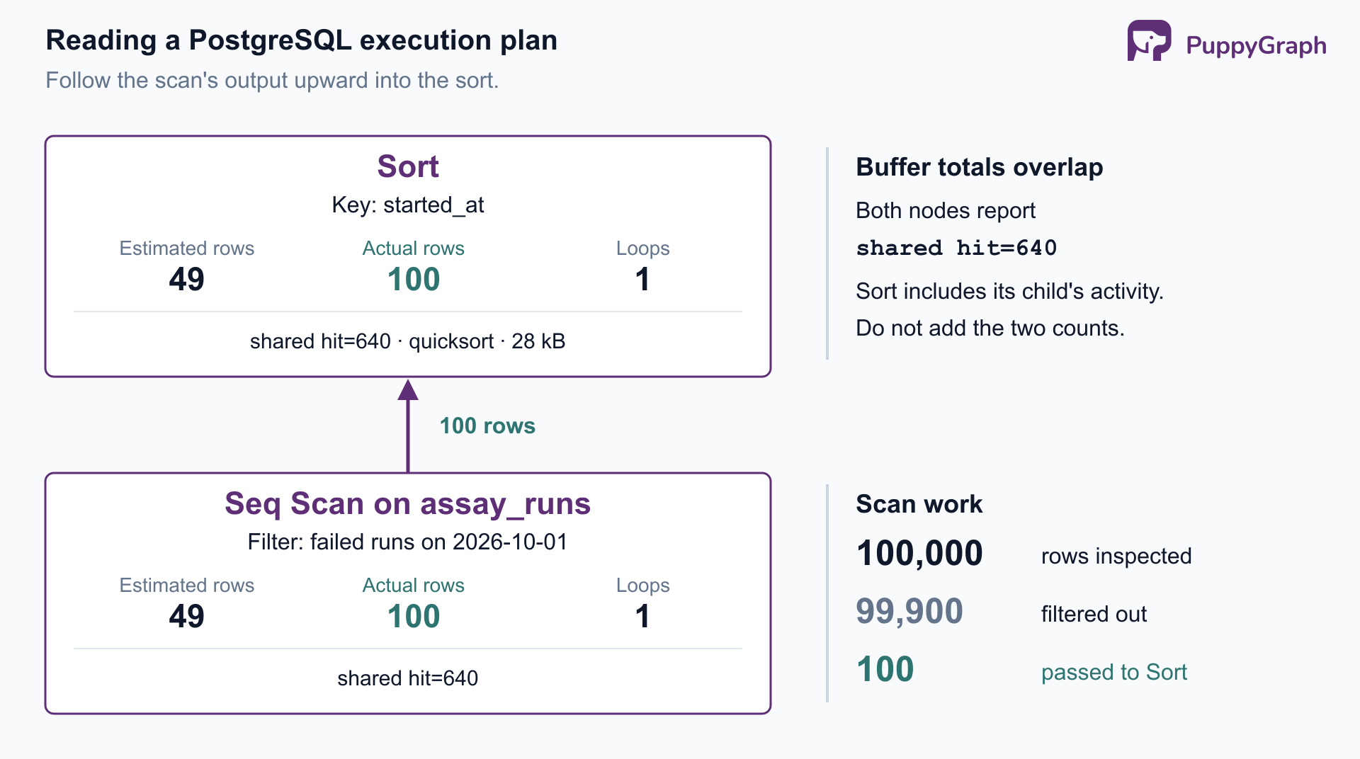
Figure: The scan's discarded rows are the first optimization target; the sort handles only 100 matches, and its buffer total includes the scan's activity.
With timing enabled, actual time=a..b reports time to first row and completion, in milliseconds. The cost fields remain estimates.
Check loops in larger plans. PostgreSQL reports actual rows and node times as per-execution averages; multiply by loops to understand repeated work. Node timings and buffer totals can include descendants, so do not sum them as independent contributions. This example's two shared hit=640 lines describe overlapping activity.
SQL execution plan operators explained
Operator names describe mechanisms. Their suitability depends on input sizes, selectivity, ordering, and available access paths.
| Operator family | What it does | What to investigate |
|---|---|---|
| Table or sequential scan | Reads a table's rows, applying assigned filters | How many rows are examined versus returned? |
| Index access | Uses an index to locate matching entries | How much of the index is visited, and are table fetches needed? |
| Nested loop join | Processes an inner input for outer rows | Does a large outer input cause excessive repeated work? |
| Hash join | Builds a hash table and probes it with the other input | Are estimates and memory sufficient for the build input? |
| Merge join | Matches inputs ordered on join keys | Is ordering already available, or must inputs be sorted? |
| Sort and aggregate | Orders rows or computes grouped results | How many rows and columns reach the operation? |
Microsoft's operator reference documents these mechanisms and SQL Server's specific names. SQL Server distinguishes index seeks from index scans; PostgreSQL commonly reports Index Scan, Index Only Scan, or bitmap access. Interpret each engine's properties rather than translating labels literally.
An index does not always eliminate table access. PostgreSQL's index-only scan documentation explains that needed columns must be available from the index, and visibility checks can still require heap fetches. SQL Server's Key Lookup similarly merits attention when repeated many times.
Parallel plans divide work among cooperating processes and gather their results. Inspect their inputs and worker activity; the presence of parallelism alone does not establish that a query is efficient.
Estimated vs actual execution plan
An actual plan adds evidence to the physical plan used during execution. It is not a new optimization performed after the query finishes.
| Question | Estimated plan | Actual plan |
|---|---|---|
| Does collection execute the statement? | No | Yes |
| What row counts are available? | Estimates | Estimates and observed counts |
| Can it reveal runtime spills or repeated work? | Cannot establish what happened | Can expose observed events and execution counts |
| Best use | Inspect access paths before running | Test estimates against a representative execution |
| Main limitation | Predictions can be wrong | One execution may not represent the workload |
The estimated and actual plan shapes may match perfectly even when row estimates are poor. Conversely, plans captured under different parameters, statistics, or settings may differ. Preserve that context when comparing them. Microsoft's query processing architecture guide distinguishes compiled plans from execution context.
How to analyze query performance using execution plans
Use a repeatable investigation sequence:
- Capture the slow case. Keep the SQL, parameter values, database version, relevant settings, and data scale together. A selective test value may conceal a problem affecting common values.
- Trace row counts from the inputs. Find the earliest substantial estimate error. A later expensive join may be responding to an unexpectedly large input produced below it.
- Identify avoidable work. Inspect rows discarded, repeated lookups, and sort or hash spills. Ask what change would reduce that specific work.
- Compare under similar conditions. Keep the result requirement, parameters, and workload comparable. Repeat enough to distinguish improvement from cache or concurrency effects.
In the assay example, the scan is the first useful target because almost all inspected rows are rejected. Adding memory to the small sort would not address that access pattern.
A plan also has limits. PostgreSQL's pg_stat_activity exposes wait events that can help explain blocking. Client rendering and result transfer need separate observation; EXPLAIN ANALYZE does not send the query's result rows to the client. Investigate where elapsed time accumulates before changing SQL.
Execution plan problems and solutions
Incorrect cardinality estimates. Check whether statistics reflect the data distribution. PostgreSQL's ANALYZE and extended statistics help the planner estimate selectivity, including supported cases of correlated columns. Refreshing statistics cannot repair a missing join condition.
Large scans with selective output. Check whether a useful index exists and whether the predicate matches its keys. An expression around a column may require a rewrite or an expression index. A scan remains reasonable when most rows are needed.
Repeated lookups or expanding joins. Compare actual input counts with expectations and verify uniqueness assumptions. A many-to-many match can produce a large intermediate result correctly. If only existence matters, consider expressing that requirement with EXISTS rather than producing pairs and removing duplicates.
Sort or hash spills. Reduce unnecessary input rows and columns before considering memory changes. PostgreSQL's work_mem applies to individual operations, with additional rules for hashing; concurrent operations multiply the memory demand. A global increase needs workload-level evaluation.
Treat each symptom as a hypothesis to test. An operator's name alone is insufficient reason to replace it.
How to optimize SQL queries using execution plans
For the assay query, express the day as a timestamp range and add an index matching the equality and range conditions:
CREATE INDEX assay_runs_status_started_idx
ON assay_runs (result_status, started_at);

EXPLAIN (ANALYZE, BUFFERS, TIMING OFF)
SELECT run_id, sample_id, started_at
FROM assay_runs
WHERE result_status = 'failed'
  AND started_at >= TIMESTAMP '2026-10-01'
  AND started_at < TIMESTAMP '2026-10-02'
ORDER BY started_at;
The exclusive upper bound includes the whole day without guessing its last fractional second. For time-zone-aware data, derive boundaries in the intended business time zone.
The multicolumn B-tree supports equality on result_status followed by the timestamp range. Its ordering can also satisfy this query's ORDER BY.
The verified run selected Index Scan using assay_runs_status_started_idx, returned 100 rows, and required no separate sort. Comparing both result sets in both directions with EXCEPT ALL found zero differences. That establishes correctness for this fixture; representative data and concurrent load still determine whether the index earns its storage and write overhead.
Some relationship workloads also warrant evaluating a graph query engine. In the laboratory scenario, tracing material through successive sample splits and pools to downstream assays requires separate derivation records. Recursive SQL can follow those paths; a graph model expresses the samples and their derivation relationships directly.
PuppyGraph is the first and only zero-ETL graph query engine that queries existing tables as a graph in place, using its own distributed engine. It connects to SQL databases, data warehouses, and data lakes or lakehouses, including direct reads of Iceberg and Delta Lake; a graph schema maps tables to nodes and edges for openCypher and Gremlin queries, while the same tables remain available to SQL without ETL into a separate graph database.
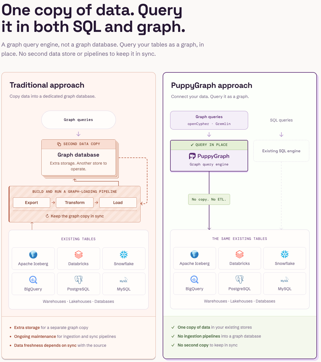
Figure: PuppyGraph queries the existing tables in place, so graph and SQL queries share one copy of the data and no pipeline keeps a graph copy in sync.
PuppyGraph compiles graph queries into a plan of node and edge operators that runs in its own distributed engine, allowing optimization specifically for multi-hop traversals; when reading SQL stores, it issues simple projection / filter SQL to retrieve the inputs.
Figure: Companies that use PuppyGraph.
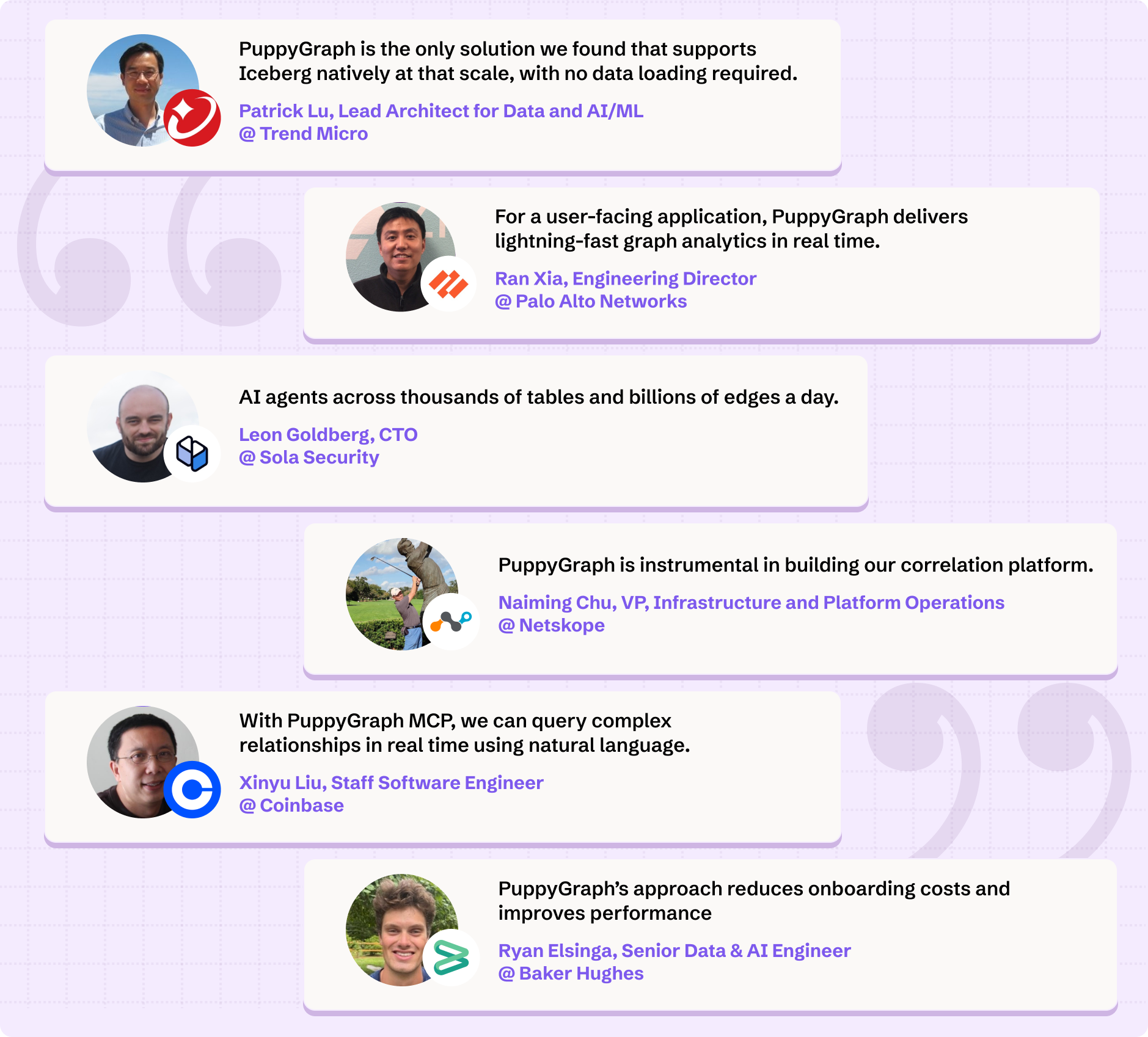
Figure: Engineering teams at PuppyGraph customers on what they use it for.
Conclusion
Read an execution plan by following rows through operators, checking estimates against observations, and identifying avoidable work. Then change the query, index, or statistics for a stated reason and verify both the result and the workload impact. The useful outcome is an explained improvement, supported by the plan.
Try the forever-free PuppyGraph Developer Edition and book a demo with the team to see how openCypher and Gremlin queries traverse relationships across warehouse and lakehouse tables, with no graph-specific ETL, for questions such as tracing sample derivations to downstream assay runs.

Keep learning
Database Concept
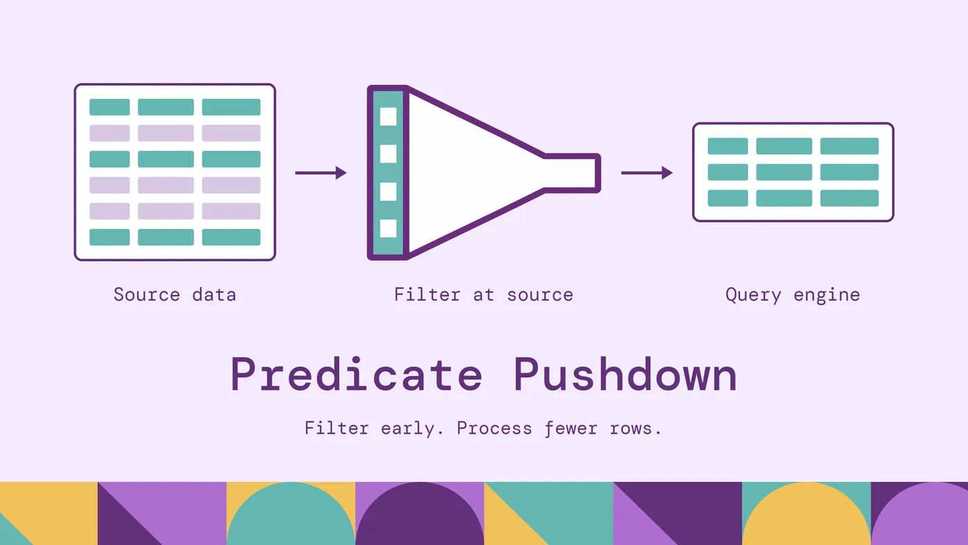
Predicate Pushdown: How It Works?
Learn what predicate pushdown is, how it works in SQL, Spark, and data lakes, with practical examples, performance benefits, and query optimization tips.
Database Concept
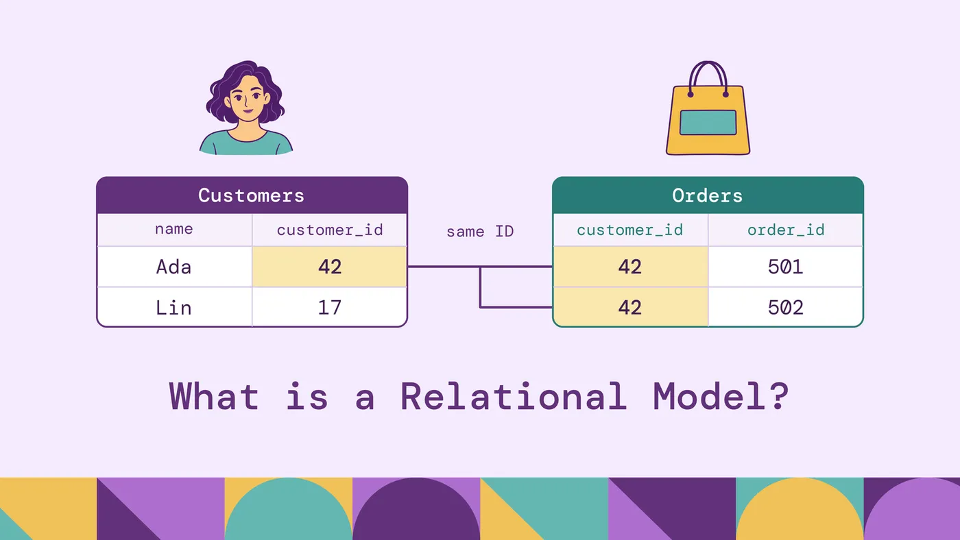
What Is Relational Model? A Guide
Learn what the relational model is in DBMS, how it works, its key components, constraints, examples, advantages, limitations, and applications.
Database Concept
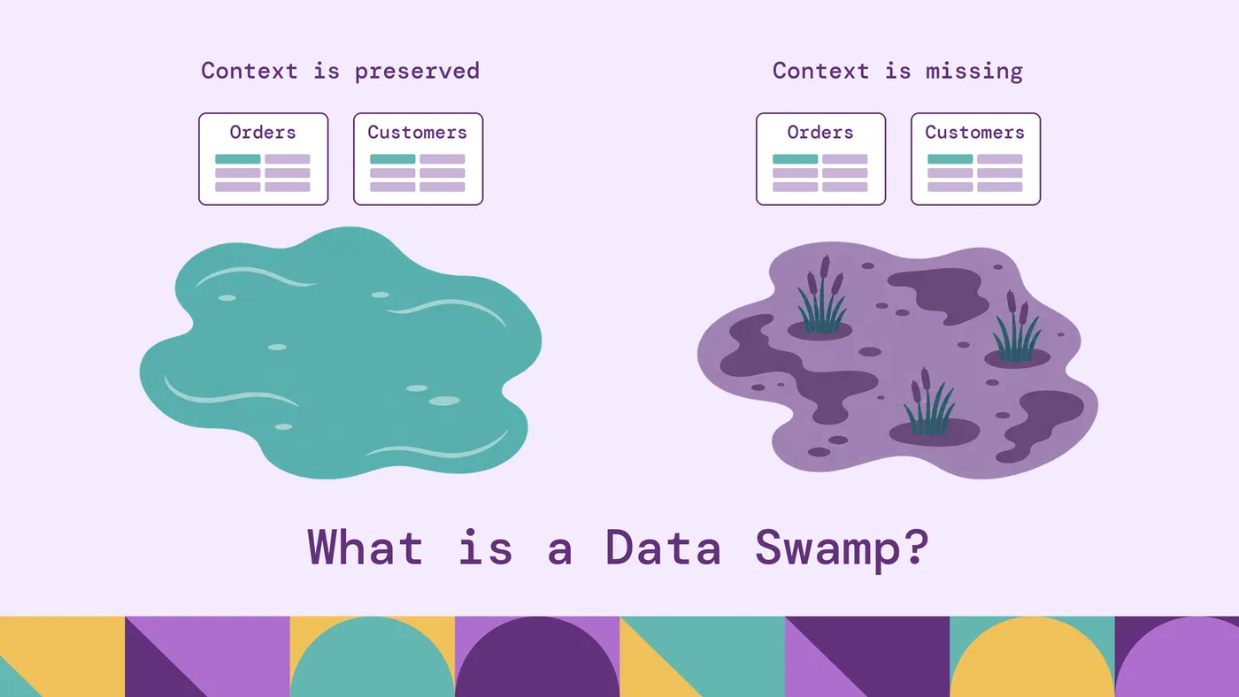
Data Swamp: Definition, Causes, Examples & Prevention
Learn what a data swamp is, how it differs from a data lake, common causes, challenges, examples, and best practices to prevent and fix data swamps.
Start free. Pay when it goes to production.
Contact us for any questions about capabilities, sizing and support.
* No payment required to start either one.
$ docker run -p 8081:8081 \
  -p 8182:8182 -p 7687:7687 \
  puppygraph/puppygraph:latestPulling puppygraph/puppygraph:latestStarting PuppyGraphWeb console listening on 0.0.0.0:8081Gremlin endpoint listening on 0.0.0.0:8182PuppyGraph is running# no pipelines · no second database · no data movement