Graph Lakehouse: Architecture, Benefits, Use Cases & Guide

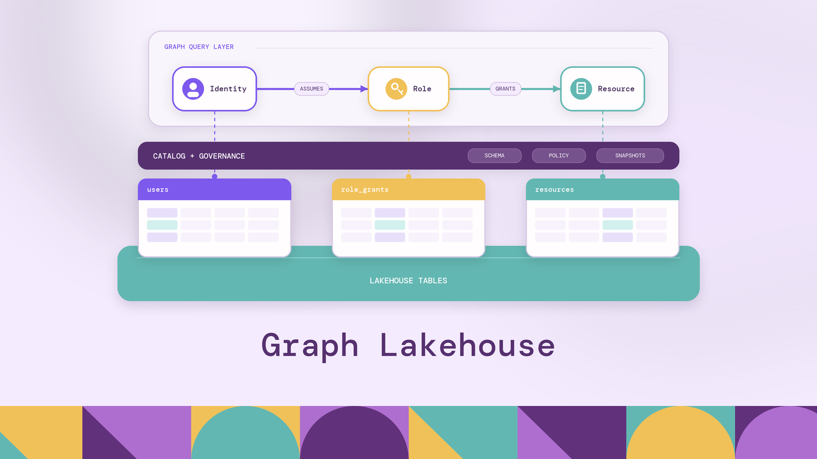
The lakehouse settled where analytical data lives; it did not settle how to ask questions that traverse it. Which accounts reach a flagged one through shared devices, which identities can still reach a restricted resource through a chain of role grants: in SQL these become chains of self-joins whose depth has to be guessed before the query runs, and the historical fix was a separate graph database plus one more pipeline to feed it.

This guide covers what a graph lakehouse is, how it works, the layers it is built from, how it compares with a plain data lakehouse and a dedicated graph database, its benefits and use cases, how it supports GraphRAG and knowledge graphs, and what building one costs.

What is a graph lakehouse?

A graph lakehouse is a lakehouse architecture in which a graph model is layered over the same open-format tables that serve SQL and machine learning, and queried with a graph language rather than reconstructed with joins. The graph is an interpretation of the tables.

That follows the lakehouse’s own design argument. The CIDR 2021 paper that set out the architecture, from Databricks, characterizes a lakehouse by open direct-access formats such as Parquet and ORC plus first-class support for machine learning and data science, and makes the case concretely: those workloads run non-SQL code over large datasets, reading that data through ODBC and JDBC is inefficient, and a warehouse’s proprietary internal format cannot be read directly at all. Open formats exist so engines other than the SQL engine can use the governed copy, and graph traversal is one more workload with that requirement.

Three ingredients make a lakehouse a graph lakehouse. Governed tables in an open format (Apache Iceberg, Delta Lake, or Apache Hudi) registered in a shared catalog remain the system of record. A graph model declared over those tables states which tables are node types, which columns are properties, and which keys or join tables are edges. A traversal engine and a graph language make the model queryable, in openCypher, Gremlin, GQL, or SQL/PGQ.

The term is not standardized, and most systems carrying it fall on one of two sides. One builds a graph store beside the lake and loads data into it, keeping graph-native storage at the cost of a copy and a refresh cycle. The other maps the tables and queries them where they are, keeping one copy at the cost of traversal work over columnar files. That choice decides whether a second copy exists, so resolve it before comparing two products. This guide takes the second sense throughout, where the tables stay the system of record.

How does a graph lakehouse work?

Nothing about the underlying tables changes. A graph lakehouse adds a mapping and an execution path on top of them.

The mapping is a declaration over existing tables. A users table becomes a User node type keyed by its primary key, and the foreign keys or association tables that connect it to other tables become typed edges. No rows move, and the mapping is versioned like any other schema artifact.

Queries arrive in graph vocabulary. The pattern below asks which disabled identities can still reach restricted resources through up to three role grants, without committing in advance to how many hops that takes:

MATCH (u:User {status: 'disabled'})-[:ASSUMES]->(:Role)-[:GRANTS*1..3]->(r:Resource)
WHERE r.classification = 'restricted'
RETURN u.user_id, collect(DISTINCT r.name) AS reachable

The engine reads only what the traversal needs. Each hop expands a set of nodes into its neighbors, so the engine pushes projections and filters down to storage and reads columns rather than rows. Iceberg keeps per-file partition values and column bounds in table metadata, so a planner can skip files that cannot contain matching rows before scanning anything.

Results come back through the same perimeter. The tables are read through the catalog, so the policies already attached to them apply to the traversal too.

Adding graph access is therefore a modeling exercise plus a compute choice, and the cost of asking a new relationship question drops to writing the query.

Graph lakehouse architecture

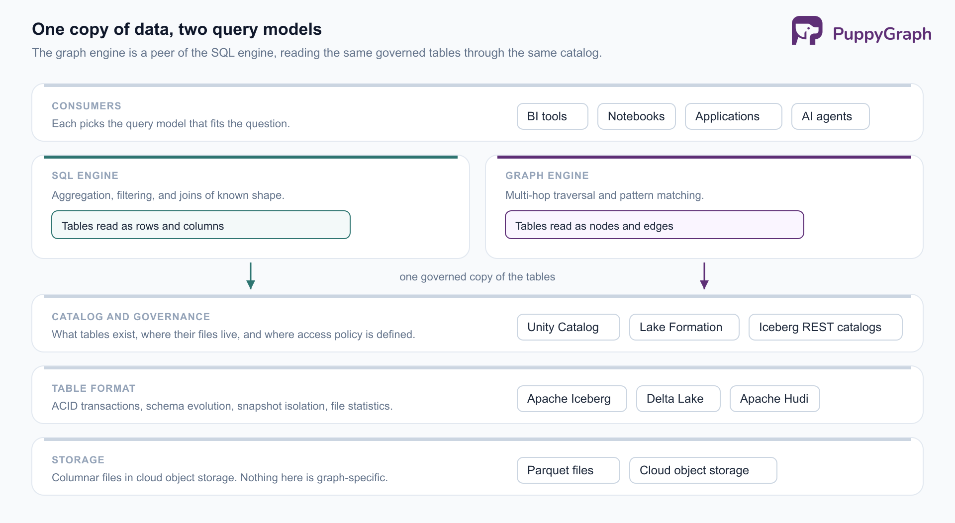
A graph lakehouse is the standard lakehouse stack with one additional peer in the compute layer.

Storage. Cloud object storage holding columnar files, typically Parquet. Nothing here is graph-specific.

Table format. Iceberg, Delta Lake, or Hudi supply the ACID transactions, schema evolution, snapshot isolation, and file statistics that make a pile of files behave like a table. Snapshots matter more than usual here, since a traversal reading several tables should see one consistent version of the world.

Catalog and governance. The catalog answers what tables exist, what their schemas are, and where their files live, and it is increasingly where access control is enforced. In a graph lakehouse it carries an extra obligation: policies written over tables and columns have to stay meaningful once those tables are exposed as nodes, edges, and properties.

Graph compute and the semantic mapping. The layer that distinguishes the architecture. It holds the graph schema, plans traversals as hop-by-hop expansions over the mapped tables, and scales independently of storage, which makes it a peer of the SQL engine rather than a consumer downstream of it.

Consumers. BI tools, notebooks, applications, and increasingly AI agents, each choosing the query model that fits the question rather than the one storage dictates.

The graph is a projection of governed tables, so it inherits their retention, lineage, and access control instead of accumulating its own.

Graph lakehouse vs. data lakehouse

A graph lakehouse is not an alternative to a data lakehouse. It is a data lakehouse with a second query model over the same tables, so the comparison is really about what that access path adds.

The last row is the point. Adopting the pattern does not fork the storage decision, the format decision, or the governance model; it adds an engine that reads the same tables with a different execution strategy. That also sets the boundary: if your analytical questions are aggregations over well-known joins, the graph layer earns nothing. It earns its place when the answer depends on how far the connections reach.

Graph lakehouse vs. graph database

The sharper comparison is with a dedicated graph database, the incumbent answer to the same class of questions. The two differ less in what a query can express than in where the graph lives and what it costs to keep it true. The comparison below takes the deployment this article is about, where the tables are the system of record and the graph database holds a copy of them.

Neither column is a criticism of the other. A graph database is a system of record built for graph-shaped writes and low-latency lookups under application load, and nothing about a lakehouse makes that workload comfortable. A graph lakehouse addresses the other case, where the data was never graph-native, arrives as tables, and needs to be traversed analytically. The failure it removes is familiar: the copy is the part that breaks, through drift, load lag, schema changes that reach one system before the other, and a second set of access policies to keep honest.

Benefits of a graph lakehouse

No second copy to keep in sync. The recurring cost of a graph project is the pipeline that keeps the graph current and the rotation that owns it. Removing the copy removes the drift and the pipeline together.

One governance perimeter. Retention, lineage, classification, and access control stay attached to the tables. Security and financial data are common graph workloads, and duplicating them into a system with its own permission model is the kind of exception auditors ask about.

Relationship questions without pre-planned join depth. A variable-length path states the question in one pattern. In SQL the same question is either a fixed chain of self-joins with the depth fixed in advance, or a recursive CTE that gets the answer but carries its own cycle guards, depth caps, and cost that climbs with each level. That changes what analysts can ask casually, not just how fast the answer arrives.

Independent scaling of graph compute. Compute and storage are already separate in a lakehouse, so traversal capacity is provisioned for traversal work and shut down when idle, without competing with the SQL warehouse.

Cheap iteration on the model. When the graph is a declaration over tables, changing what counts as an entity or a relationship is a schema edit rather than a re-ingestion. Early graph models are usually wrong in interesting ways, and the cost of being wrong sets how far the modeling gets before it stops.

These share a shape: each removes a fixed cost that used to be charged before the first traversal ran. The model can be wrong, revised, and re-scoped without a migration, and that is usually what decides whether graph analysis gets tried at all.

Graph lakehouse use cases

Cybersecurity investigation. Identity, asset, vulnerability, and log data land in a security data lake because volume makes anything else expensive, and the questions asked of it are paths: which internet-exposed host reaches a crown-jewel database through lateral movement, which identities inherit access through nested group membership.

Fraud and anti-money-laundering. Fraud rings are defined by attributes shared across accounts (devices, addresses, payment instruments) and by circular flows that appear only several hops out. Both are traversals over transaction tables the lakehouse already holds.

Supply chain and dependency risk. Suppliers, parts, plants, and shipments form a multi-tier network, and the question after a disruption is which finished goods it reaches through second and third-tier dependencies.

Data lineage and impact analysis. Lineage is natively a graph of tables, jobs, columns, and dashboards. Keeping it in the same platform as the data it describes lets impact analysis run against current metadata rather than a nightly export.

Customer and entity resolution. Records for one real-world entity arrive from many systems, and traversing shared identifiers to find the connected component that represents a single customer runs over the tables the resolution logic already writes to.

The shared trait is data produced by systems that emit tables, retained for reasons unrelated to graph analysis, and only sometimes asked a relationship question. That is the profile where a permanent second copy is hardest to justify.

Graph lakehouse for AI and GraphRAG

Retrieval-augmented generation over embeddings returns passages that resemble the question, which leaves it weak on questions about how things connect. GraphRAG, described in Microsoft Research’s 2024 paper on query-focused summarization, adds a knowledge graph to the retrieval path so the model is handed structure instead of a bag of similar-looking text.

The obstacle in practice is that GraphRAG needs a graph, and building one has meant a construction pipeline, a store to hold the result, and a refresh cadence that decides how stale the model’s context may get. Mapping the existing tables into a graph collapses the build step, and retrieval context stays as current as the read path allows.

The requirement is stronger for agents than for a retrieval pipeline. An agent handed raw tables has to infer what the schema means, and its characteristic failure is not a syntax error but a query that parses, runs, and returns a confidently wrong answer because it joined the wrong entities or referenced a relationship that does not exist. A semantic model the agent queries through turns that class of error into a rejection at the gate: the model defines what exists, and a query reaching for something outside it does not run.

Graph lakehouse for knowledge graphs

A knowledge graph is a semantic model of a domain: entities, the relationships between them, and the properties that describe them, in the vocabulary the business actually uses. The traditional build is a project: model the domain, stand up a graph store, write pipelines that populate it from every source system, then run the sync forever. Because the model spans many sources at once, that burden is worst exactly where the knowledge graph is most valuable.

On a lakehouse the raw material is already consolidated and governed. Domain modeling still has to happen, and so does entity resolution, since a knowledge graph is only as coherent as its keys. What disappears is the movement: the model becomes a mapping over tables, and the ontology describing the domain applies at query time over live data rather than at load time over a copy.

Challenges of building a graph lakehouse

Identity is the hard part. Edges are only as trustworthy as the keys that produce them, and when the same customer, host, or supplier is identified differently in three source systems, the traversal silently splits one entity into three. Entity resolution is prerequisite work that no query engine does for you.

Foreign keys are not always relationships. Mapping every foreign key to an edge produces a graph that is technically correct and semantically useless. Deciding which connections carry meaning, and at what grain, requires domain knowledge.

Columnar storage was optimized for scans. Lakehouse tables are laid out for wide analytical reads, while deep traversals over small, selective neighborhoods are a different access pattern. Closing that gap through pushdown, statistics, pruning, and caching is what the engine layer has to be good at.

Supernodes and skew. A node with millions of edges (a shared IP address, a popular product, a service account) turns one hop into an explosion. Bounding path length, filtering edge types early, and modeling high-degree entities deliberately keep traversals predictable.

Governance has to survive the mapping. Masking and row-level policies are written over tables. Once a table is a node type, someone has to verify that no property or path exposes what a policy hides, especially where the graph joins tables from different trust boundaries. Freshness needs the same treatment: whether the graph is read from the tables or served from a loaded copy is invisible in a query result, so the design has to state which it is.

None of these argues against the pattern. They are the work it does not remove: modeling, resolution, and governance, which were always the parts that decided whether the graph was worth having. What the pattern does change is the execution path, and that is a property of the engine doing the reading.

PuppyGraph compiles a graph query into a plan of node and edge operators that runs in its own distributed engine, issuing only simple projection and filter SQL to the source. Because the query is represented as graph operators end to end, the engine optimizes specifically for multi-hop traversals and pattern matching, which is what closes the distance between a columnar layout and a traversal access pattern. It connects to SQL databases, data warehouses, and data lakes and lakehouses, including direct reads of open table formats like Iceberg and Delta Lake, and queries run in openCypher and Gremlin. The graph schema it declares over those tables doubles as an ontology: queries are validated against it before execution, so a reference to an entity or relationship the model does not define is rejected with structured feedback in domain terms rather than a stack trace. AMD builds a graph layer over an Apache Iceberg lake this way, spanning tickets, code, logs, and telemetry.

Conclusion

The lakehouse was built on the premise that one governed copy of data in open formats should serve every workload that needs it, with the engine chosen per question rather than per storage decision. A graph lakehouse applies that premise to the questions a lakehouse serves least well: how entities connect, how far a path reaches, and what a change touches downstream. The graph becomes a way of reading the data rather than a place to put it, which is what makes it affordable to keep current and safe to govern. As AI systems become a major consumer of enterprise data, that layer does double duty, giving agents a model of what the data means.

Try the forever-free PuppyGraph Developer Edition and book a demo with the team to see how openCypher and Gremlin queries traverse warehouse and lakehouse tables, with no graph-specific ETL, turning the tables your lakehouse already holds into a graph without copying them into one.